

An empty AVERAGEIFS is #DIV/0!, and a wrapper that turns it into 0 looks like a real average of zeros
Updated
AVERAGEIFS(average_range, criteria_range1, criterion1, …) averages numbers on rows that pass every test. If no numeric cell passes, the count you divide by is zero and the cell is #DIV/0!. It is not 0. A group whose amounts are actually 0 averages to 0, and that 0 is a successful average. Those two outcomes are different until someone wraps the function. =IFERROR(AVERAGEIFS(...),0) turns the missing group into 0. The grid then matches the real average of zeros. There is no triangle on either cell. MINIFS and MAXIFS do return 0 when nothing matches. Copying that expectation onto AVERAGEIFS is how the wrapper gets added.
Sheet Error is an independent formula-error library, not a Google product. One criterion and the same #DIV/0! is AVERAGEIF #DIV/0!. A criteria range of the wrong height is AVERAGEIFS range size, and that token is #VALUE!. MINIFS of a missing region really is 0. That page is MINIFS / MAXIFS no match. Keep the Google Sheets UI in English.
Recreate it on a blank sheet
Section titled “Recreate it on a blank sheet”- Open a blank spreadsheet. In A1 type
region, B1amt. A2East, B20. A3East, B30. A4West, B410. A5West, B530. East’s amounts are zeros. There is no North row.
A real average of zeros. In D1 type east. In D2 enter =AVERAGEIFS(B2:B5,A2:A5,"East"). D2 is 0. The rows exist. The amounts are 0. ISNUMBER(D2) is TRUE. There is no triangle. That zero is the average. Leave it.
No such region. In F1 type north. In F2 enter =AVERAGEIFS(B2:B5,A2:A5,"North"). F2 is #DIV/0!. The tooltip is the divide-by-zero error, the same family as divide by zero and AVERAGEIF #DIV/0!. North is not on the sheet. Leave F2 broken. It does not say 0.
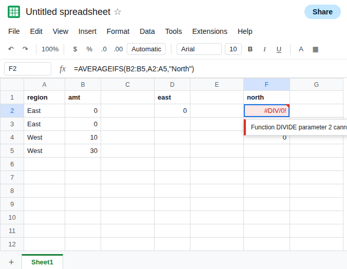
The wrapper that invents the zero. In F4 enter =IFERROR(AVERAGEIFS(B2:B5,A2:A5,"North"),0). F4 is 0. It matches D2. Nothing in F4 says the region was missing. Leave F4 as 0. In F5 enter =IFERROR(AVERAGEIFS(B2:B5,A2:A5,"North"),""). F5 looks blank. A chart will treat that string differently from #DIV/0!. See IFERROR empty string. The numeric lie is F4.
MINIFS really is 0 on the same miss. In H2 enter =MINIFS(B2:B5,A2:A5,"North"). H2 is 0. That is MINIFS / MAXIFS no match. H2 and F4 look alike. H2 did not need IFERROR. F2, unwrapped, does not look like H2. Do not copy the min formula onto an average and expect the same token.
Count the rows. In H4 enter =COUNTIFS(A2:A5,"East"). H4 is 2. In H5 enter =COUNTIFS(A2:A5,"North"). H5 is 0. The averages are not the same kind of zero. The counts are how you tell D2 from F4.
What is actually wrong
Section titled “What is actually wrong”- No numeric match means the average’s denominator is zero. Sheets returns
#DIV/0!. A blog that says the empty average “returns 0” is describingMINIFS, or describing anIFERRORsomeone already added. The raw function is F2. - Real zeros match the criteria and average to
0. Blank amounts are skipped, not treated as zero. If East’s cells were blank instead of0, D2 would be#DIV/0!too, because no numeric amount matched. A stored0is a number. See IF blank vs 0. IFERROR(..., 0)replaces#DIV/0!,#VALUE!,#N/A, and#REF!with the same0. A wrong-sized range is#VALUE!. The wrapper turns that into0as well, so a size bug and a missing region and a real zero average all look identical. See IFERROR hides cause and AVERAGEIFS range size.N()of a text label is0, andNdoes not turn#DIV/0!into a diagnostic. Do not pass the error throughNto “coerce the average.” See N() text to 0.AVERAGEIFSwith the criteria range first, the waySUMIFis written, is a different mistake. The average range is first, likeSUMIFS. See SUMIFS argument order.
Leave F2 as #DIV/0! and F4 as the false 0. Leave D2 as the real 0.
Test the count, then average. In J2 enter =IF(COUNTIFS(A2:A5,"North")=0,"no rows",AVERAGEIFS(B2:B5,A2:A5,"North")). J2 is no rows. In J3 enter =IF(COUNTIFS(A2:A5,"East")=0,"no rows",AVERAGEIFS(B2:B5,A2:A5,"East")). J3 is 0. The zero remains only when East has rows. A blank amount column that matches the region still makes AVERAGEIFS return #DIV/0! inside the IF once the count of labels is nonzero. That is “rows, but nothing numeric,” which you can split with COUNT of the amounts if you need it. The label count is enough to separate North from East on this sheet.
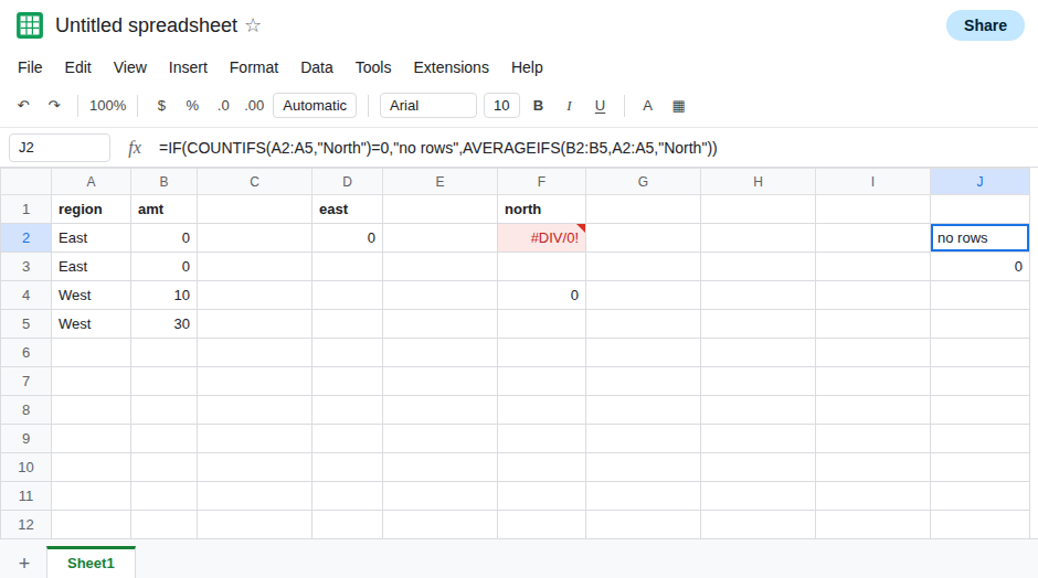
If the empty group should stay an error, delete the IFERROR and let F2 show #DIV/0!. A chart that must gap there can use NA() only after you have decided a missing region is a gap and not a zero month. See chart error gaps.
Do not add IFERROR to make F2 match H2. MINIFS and AVERAGEIFS do not share this result. See MINIFS / MAXIFS no match.
If the cell is #DIV/0!, no numeric value matched. If the cell is 0 and COUNTIFS of the same criteria is 0, a wrapper invented the zero. If COUNTIFS is greater than 0 and the average is 0, the matched amounts are zeros. If the tooltip says the arrays differ in size, you are on the size page, not this one.