

Fix QUERY “Unable to parse query string” in Google Sheets (quotes, dates, Col vs letter)
Updated
QUERY can land as #VALUE! with Unable to parse query string for Function QUERY parameter 2. The formula parsed as a Sheets formula. The query language inside the string did not. Three usual causes: a text literal without single quotes, a date without date 'yyyy-mm-dd', and Col1 vs A on the wrong kind of data.
This is not QUERY Col1 vs A. That page is IMPORTRANGE with select A, which is often #N/A. This page is the parse tooltip on a blank sheet.
Recreate it on a blank sheet
Section titled “Recreate it on a blank sheet”- Open a blank spreadsheet. In A1 type
sku, B1name, C1shipped. A2101, B2Widget. In C2 type2024-01-15so Sheets stores a real date. A3102, B3Gadget. In C3 type2024-02-01as a real date.
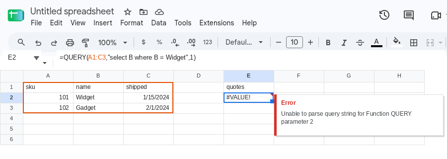
Quotes. In E1 type quotes. In E2 enter =QUERY(A1:C3,"select B where B = Widget",1). The cell shows #VALUE!. The tooltip starts Unable to parse query string for Function QUERY parameter 2. Widget is an identifier there, not a string.
Dates. In E4 type dates. In E5 enter =QUERY(A1:C3,"select B where C > 2024-01-01",1). The cell shows #VALUE!. Same tooltip family. 2024-01-01 is not a QUERY date literal.
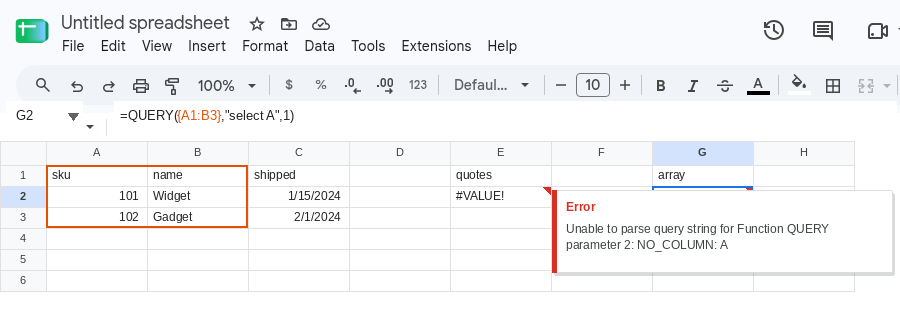
Col vs letter. In G1 type array. In G2 enter =QUERY({A1:B3},"select A",1). The cell shows #VALUE!. The tooltip is Unable to parse query string for Function QUERY parameter 2: NO_COLUMN: A. {A1:B3} is an array. Arrays do not have column letters.
In G4 type sheet. In G5 enter =QUERY(A1:B3,"select Col1",1). The cell shows #VALUE!. The tooltip is NO_COLUMN: Col1. A1:B3 is a sheet range. Sheet ranges use A, B, not Col1.
Leave E2, E5, G2, and G5 as the broken formulas.
What is actually wrong
Section titled “What is actually wrong”- The second argument is a QUERY statement, not a Sheets formula. String literals inside it use single quotes:
where B = 'Widget'. UnquotedWidgetis a parse error. PuttingWidgetin double quotes inside a double-quoted formula string usually breaks the Sheets formula first (#ERROR!/ Formula parse error) before QUERY runs. See locale parse error only if the tooltip is Formula parse error from commas vs semicolons — that is a different#ERROR!. - Date filters need the
datekeyword and ayyyy-mm-ddliteral:where C > date '2024-01-01'. A bare2024-01-01does not parse.where C > '2024-01-01'is a text comparison, not a date comparison. Concatenating a date cell with"where C > "&D1injects a serial number and fails the same way. QUERYnames columns from the first argument’s shape. A plain rangeA1:C3uses lettersA,B,C. An array{A1:B3},{A:A,C:C},FILTER(...), or anotherQUERY(...)usesCol1,Col2, … from the left of that array. Mixing them isNO_COLUMNin the parse tooltip.IMPORTRANGEis also an array (Col1,Col2). On that wrapper,select Ais commonly#N/A, not this#VALUE!parse cell. That case is Col1 vs A.
This is not mixed types in a date column. year(A) on dates mixed with TBD is also Unable to parse query string, but the tooltip is Can’t perform the function year on a column that is not a Date or a DateTime column. That page is mixed dates.
This is not #N/A from a lookup miss. See what #N/A means.
This is not COUNTIFS or SUMIFS ranges of different size. That #VALUE! tooltip is Array arguments to COUNTIFS are of different size. See COUNTIFS range size.
Leave the four broken cells so the parse errors stay on the sheet.
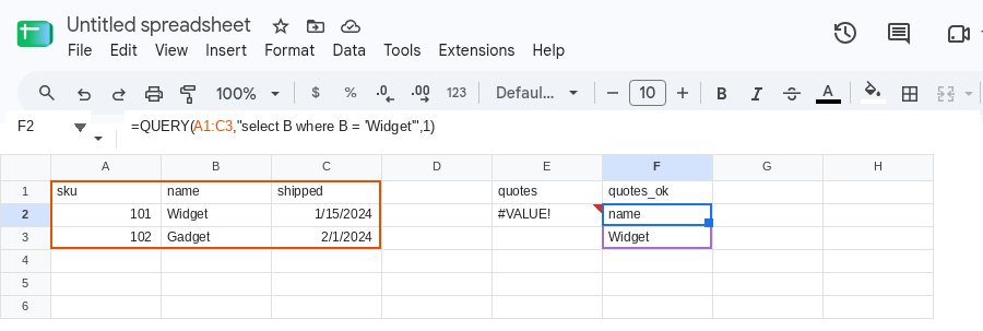
Quote the text literal. In F1 type quotes_ok. In F2 enter =QUERY(A1:C3,"select B where B = 'Widget'",1). The formula spills name / Widget. To pull the criterion from a cell: =QUERY(A1:C3,"select B where B = '"&B2&"'",1) — close the double-quoted fragment, concatenate, reopen. Do not drop the single quotes around the value.
Write a date literal. In F4 type dates_ok. In F5 enter =QUERY(A1:C3,"select B where C > date '2024-01-01'",1). The formula spills name / Widget / Gadget. From a date in D5: =QUERY(A1:C3,"select B where C > date '"&TEXT(D5,"yyyy-mm-dd")&"'",1). TEXT(...,"yyyy-mm-dd") is required. TODAY() in the query string is not a substitute for that literal.
Match Col vs letter to the data. In H1 type array_ok. In H2 enter =QUERY({A1:B3},"select Col1",1). The formula spills sku / 101 / 102. In H4 type sheet_ok. In H5 enter =QUERY(A1:B3,"select A",1). Same spill. {A1:B3} → Col1. A1:B3 → A. Do not mix.
Do not wrap this #VALUE! in IFERROR and call the query fixed. Do not change File > Settings locale to repair quotes or date '...'. Do not switch to IMPORTRANGE to “make Col1 work” — pick the names that match the argument you already have.
If the tooltip is Unable to parse query string, read the rest of the tooltip: PARSE_ERROR near an unquoted word, an invalid date literal, or NO_COLUMN. Fix that token. The Sheets formula bar can look valid the whole time.