Fix #N/A after a CSV import in Google Sheets (text vs number)

A CSV import can store the same id as a number in the table and as text in the lookup (or the reverse). VLOOKUP with FALSE does not coerce them. The cell is #N/A. The row is on the sheet. You can still see 101 in both places.

This page is the import type split. It is not what #N/A means (the key is absent) and not VLOOKUP no match (typed apostrophe vs number, or a trailing space). If LEN shows a leftover space, use that page. If the sku is not in the column at all, use the primer.

Recreate it on a blank sheet

You do not need a file. Build the columns the way File → Import → Upload leaves them when Convert text to numbers, dates, and formulas is on (the usual default).

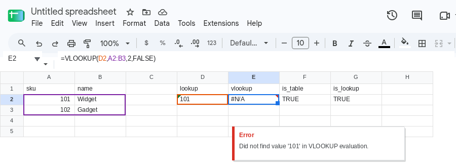
1. Open a blank spreadsheet. In A1 type sku, B1 name. This block is the imported table.
2. In A2 type 101 as a number. B2 Widget. In A3 type 102 as a number. B3 Gadget. Sheets did this to CSV fields that looked numeric.
3. In D1 type lookup, E1 vlookup, F1 is_table, G1 is_lookup. In D2 type an apostrophe then 101 so the cell is text — the id as it still appears in the form, the other CSV, or a paste that stayed text. In E2 enter =VLOOKUP(D2,A2:B3,2,FALSE). The cell shows #N/A. The tooltip is Did not find value ‘101’ in VLOOKUP evaluation.
4. In F2 enter =ISNUMBER(A2). The cell shows TRUE. In G2 enter =ISTEXT(D2). The cell shows TRUE. Same digits. Different types.

E2 selected. Formula bar shows =VLOOKUP(D2,A2,2,FALSE). E2 is #N/A. Tooltip: Did not find value '101' in VLOOKUP evaluation. F2 is TRUE. G2 is TRUE.

5. Leading zeros. CSV 00101 becomes 101 when converted. In A5 type sku_pad, B5 name. In A6 type 101 as a number. B6 Bolt. In D5 type lookup_pad. In D6 type an apostrophe then 00101. In E6 enter =VLOOKUP(D6,A6:B6,2,FALSE). The cell shows #N/A. A6 is the number 101. D6 is the five-character string 00101.

E6 selected. Formula bar shows =VLOOKUP(D6,A6,2,FALSE). E6 is #N/A. Tooltip: Did not find value '00101' in VLOOKUP evaluation. D6 is text 00101. A6 is number 101.

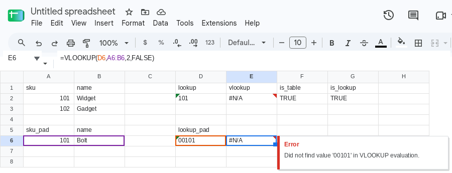
Leave E2 and E6 as the broken formulas.

What is actually wrong

• File → Import infers types per column. A sku column of 101, 102, 103 becomes numbers. A lookup you type, paste from a ticket, or import from a second file that had mixed ids stays text ('101). VLOOKUP, MATCH, and XLOOKUP with an exact match do not treat those as equal.
• Leading zeros are dropped when the field becomes a number. The table no longer holds 00101. A lookup of 00101 cannot hit 101.
• The error value is still #N/A. That does not mean the row is missing. ISNUMBER / ISTEXT on the two key cells is the check.
• A trailing space is a different mismatch. LEN on both keys. If the lengths disagree and you did not expect padding, see VLOOKUP no match.

This is not #VALUE!. #VALUE! is a wrong type in arithmetic (10 + pcs). See wrong type. The lookup ran. The keys did not match.

This is not a Formula parse error. See locale parse error.

Fix

Leave E2 and E6 broken so #N/A stays on the sheet.

Confirm the types. F2 TRUE and G2 TRUE already show number table vs text lookup. If both ISNUMBER, you are not on this page. If both ISTEXT and you still miss, check spaces on the VLOOKUP page.

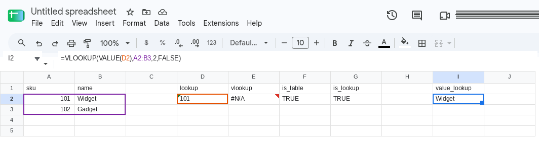
Make the lookup a number when the table is numbers. In I1 type value_lookup. In I2 enter =VLOOKUP(VALUE(D2),A2:B3,2,FALSE). The cell shows Widget. In I6 enter =VLOOKUP(VALUE(D6),A6:B6,2,FALSE). The cell shows Bolt. VALUE("00101") is 101, which is what the import stored.

I2 selected. Formula bar shows =VLOOKUP(VALUE(D2),A2,2,FALSE). I2 is Widget. E2 is still #N/A.

Make the table text when the lookup is text. Use this when you must keep leading zeros. Re-import will not bring zeros back if the column is already numeric — the zeros are gone. For a text lookup of 101 against numeric 101: in K1 type text_table. In K2 enter =VLOOKUP(D2,ARRAYFORMULA({TO_TEXT(A2:A3),B2:B3}),2,FALSE). The cell shows Widget. TO_TEXT(101) is 101, which matches '101. It does not match '00101. For padded ids, format the sku column as Plain text and import again with Convert text to numbers, dates, and formulas off, so 00101 stays 00101.

Convert the imported column once. In M1 type sku_num. In M2 enter =ARRAYFORMULA(VALUE(A2:A3)). Then look up against that helper, not against A. Prefer one helper column over wrapping VALUE in every lookup.

Fix it at import when you still have the file. File → Import → Upload. Uncheck Convert text to numbers, dates, and formulas if the ids must stay codes (leading zeros, long digit strings). Or pre-format the destination column as Plain text, then paste. Do not rely on a leading apostrophe in the CSV; most importers will not keep it.

Do not wrap E2 in IFNA until the types match. IFNA will print “none” for a miss that is really 101 vs '101. See what #N/A means. If changing D2 from '101 to the number 101 makes Widget appear, the function is working and the import type is the bug.