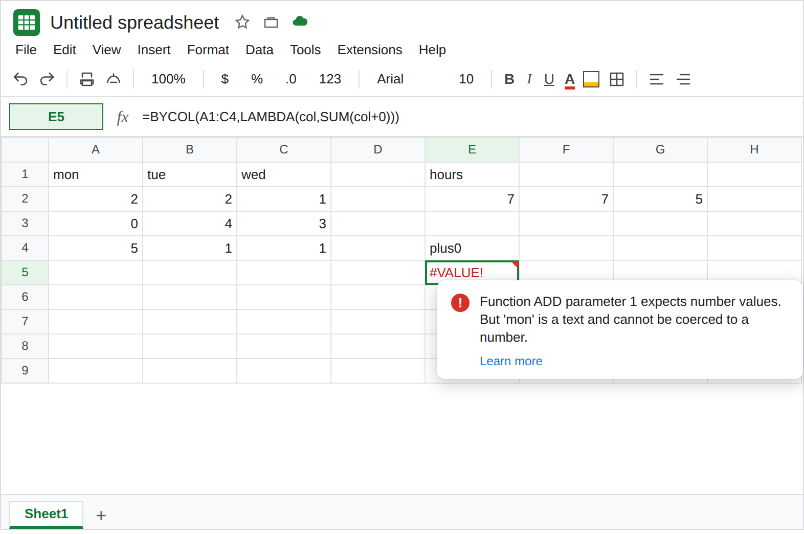
BYCOL includes the header row and returns #VALUE!

BYCOL runs a LAMBDA once per column of the range you pass. If that range starts on row 1, the header is part of the column. mon is text. SUM(col+0) tries to add that text and the cell is #VALUE!. The hours underneath never get a total. A lambda that only SUMs the column can ignore text and still divide by the header row, so the average is too small and there is no triangle.

Returning the column array is BYCOL LAMBDA (Single value expected). This page is the header sitting inside an otherwise numeric column. Keep the Google Sheets UI in English. Helper names stay English: LAMBDA, BYCOL.

Recreate it on a blank sheet

1. Open a blank spreadsheet. In A1 type mon, B1 tue, C1 wed. A2 2, B2 2, C2 1. A3 0, B3 4, C3 3. A4 5, B4 1, C4 1. Column totals of the hours are 7, 7, and 5. The headers are not hours.

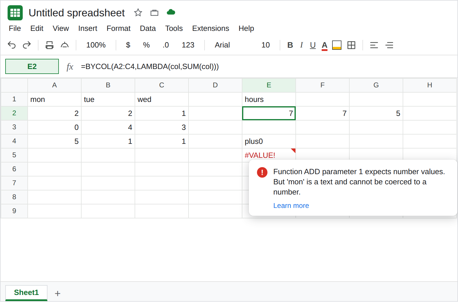
The numeric block. In E1 type hours. In E2 enter =BYCOL(A2:C4,LAMBDA(col,SUM(col))). The spill is a row: E2 7, F2 7, G2 5. That row is the control. The range started on row 2.

Coerce the header. In E4 type plus0. In E5 enter =BYCOL(A1:C4,LAMBDA(col,SUM(col+0))). The range is A1:C4. Each column begins with mon, tue, or wed. col+0 requires numbers. The cell shows #VALUE!. The tooltip says a parameter expects number values and names the text (mon or the header it hits first). Leave E5 broken.

A quiet wrong average. In E7 type rows. In E8 enter =BYCOL(A1:C4,LAMBDA(col,SUM(col)/ROWS(col))). SUM skips text, so the numerator is 7, 7, 5. ROWS counts the header. Each column is 4 rows. The spill is 1.75, 1.75, 1.25, not 7/3. There is no error triangle. Leave E8 as those three small numbers. They are not the hour averages.

AVERAGE on the same header range. In E10 enter =BYCOL(A1:C4,LAMBDA(col,AVERAGE(col))). AVERAGE skips text. The spill matches the true hour averages (7/3, 7/3, 5/3) even though row 1 was included. That success does not make E5 legal, and it does not make E8’s divisor right. Leave E10 as the contrast: skipping text is not the same as “I started below the header.”

What is actually wrong

• BYCOL does not know that row 1 is a label. A1:C4 is four rows. The lambda receives mon then 2, 0, 5 as one column.
• +0 is numeric coercion. Text fails it. The tooltip is a type error, the same family as wrong type. E2 never added the header, so E2 is 7.
• SUM and AVERAGE skip text. They will not save col+0. They will also not tell you that ROWS(col) counted mon. E8 is the silent miss. E5 is the loud one.
• Open columns keep the header too. A1:C is every row, including row 1 and a long tail of blanks. SUM of blanks is 0. The header problem remains. Bound the range.
• Two lambda names, or returning col, is BYCOL LAMBDA. E5 has one name and tried to return one sum. The sum’s input is the bug.

Fix

Leave E5 as #VALUE!. Leave E8 as 1.75 / 1.75 / 1.25.

Start on the first hour. Keep E2: =BYCOL(A2:C4,LAMBDA(col,SUM(col))). 7, 7, 5. For a mean of those hours, =BYCOL(A2:C4,LAMBDA(col,AVERAGE(col))) uses three numbers, not four rows.

If the header must stay inside the range, drop it inside the lambda with a numeric test: =BYCOL(A1:C4,LAMBDA(col,SUM(FILTER(col,ISNUMBER(col))))). The spill matches E2. FILTER on an all-text column returns #N/A, so do not point this at a notes column. See FILTER no match.

Do not wrap E5 in IFERROR. The header is still in the range and the totals become blanks. See IFERROR vs IFNA.

If BYCOL is #VALUE! and row 1 is text, start the range on the first number, or filter to ISNUMBER. If the cell is a small average with no triangle, check whether ROWS counted the header.