HLOOKUP with TRUE on an unsorted header row returns the wrong column

HLOOKUP(key, range, row, TRUE) reads the first row as sorted breaks, left to right, and returns the rightmost header that is still less than or equal to the key. Omit the fourth argument and Sheets uses TRUE. On a header typed out of order, that call is #N/A or a price from a different column, with no triangle when it hits the neighbor. FALSE on the same key returns the column whose header is exactly 30.

A missing header such as 999, and a row index past the range, are HLOOKUP #N/A / #REF!. The vertical form of this band is VLOOKUP TRUE bands. Keep the Google Sheets UI in English. Sheet Error is an independent formula-error library, not a Google product.

Recreate it on a blank sheet

1. Open a blank spreadsheet. In A1 type qty. B1 40, C1 10, D1 30, E1 20. In A2 type price. B2 8, C2 3, D2 6, E2 5. The headers are not sorted. The price under 30 is 6, in column D.

Exact. In G1 type key. G2 30. In I1 type exact. In I2 enter =HLOOKUP(G2,B1:E2,2,FALSE). The cell shows 6. Row index 2 is the price row. FALSE requires an equal header. I2 is the control.

Approximate on the same unsorted row. In I4 type approx. In I5 enter =HLOOKUP(G2,B1:E2,2,TRUE). I5 is #N/A or a price that is not 6. Both are wrong for a header that I2 already found. If I5 shows 8, 3, or 5, that number belongs to another column, and there is no error triangle. Do not treat it as the band for 30. Leave I5 as whatever it shows when it is not 6.

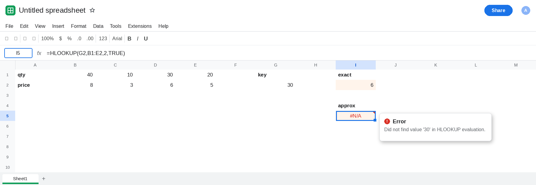
The default is TRUE. In I7 enter =HLOOKUP(G2,B1:E2,2). No fourth argument. I7 matches I5, not I2. Leave I7 beside I5.

A sorted header, so TRUE has a place. In B5 type 10, C5 20, D5 30, E5 40. B6 3, C6 5, D6 6, E6 8. This header ascends. In K2 enter =HLOOKUP(25,B5:E6,2,TRUE). The cell shows 5. Header 20 is the largest break that is still <= 25, and the price under it is 5. In K3 enter =HLOOKUP(25,B5:E6,2,FALSE). K3 is #N/A. 25 is not a header. FALSE is supposed to fail there. TRUE is the band. Leave K2 as 5 and K3 as #N/A.

Leave I5 and I7 as the unsorted approximate results. Leave I2 as 6. Leave K2 as 5.

What is actually wrong

• The fourth argument defaults to TRUE. A formula copied from a column of breaks onto a header row silently stops being exact. I7 is that copy, turned sideways.
• TRUE does not mean “closest header.” It means a sorted ascending search along row 1 of the range. B1:E1 goes 40, then 10, then 30. The contract is already false. The result is #N/A or some other price.
• A wrong price with no triangle is the case a dashboard will sum. #N/A at least looks unfinished. Check I5 against I2 before you ship a number.
• The row index is still a row index. 2 means the second row of B1:E2, not “column 2.” A 3 on this two-row range is #REF!, which is HLOOKUP #N/A / #REF!. I5’s range has the row it asked for.
• Vertical VLOOKUP with TRUE is the same approximate rule on a column. See VLOOKUP TRUE bands. MATCH type 1 is the position form. See MATCH approx unsorted.

This is not an exact miss of a header that is not on the row. =HLOOKUP(999,B1:E2,2,FALSE) is #N/A because 999 is absent. G2 is 30, and I2 found it.

Fix

Leave I5 and I7 unsorted and approximate.

Exact headers use FALSE. Keep I2. In I9 enter =HLOOKUP(G2,B1:E2,2,FALSE) if you want the repair in a fresh cell. It shows 6. XLOOKUP across the header is exact by default: =XLOOKUP(G2,B1:E1,B2:E2) in I11 is also 6.

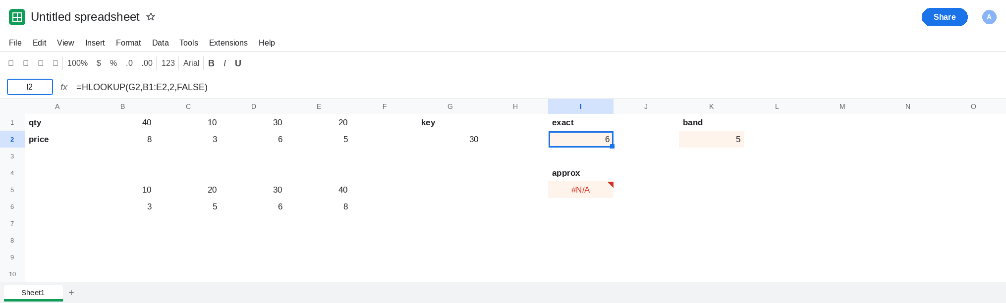
Approximate only on a sorted header. Keep K2 as the pattern. Leave B5:E5 ascending. Do not point K2 at B1:E1 to avoid sorting.

Do not wrap I5 in IFNA while it might be a wrong price. IFNA only hides the #N/A branch. See IFERROR vs IFNA.

If HLOOKUP returns a price and FALSE on the same key returns a different price, the fourth argument is TRUE or it was omitted. Pass FALSE for an exact header. If the header is a sorted row of breaks, TRUE belongs on that row, on the same terms as the VLOOKUP TRUE page.