Pivot Show as % of column snaps back to the raw sums

A pivot value has a Show as setting that is separate from the summarizer and separate from a percent format on the source. % of column divides each row by the column total. East 30, West 10, North 10 become 60%, 20%, and 20%. % of row, when that value is the only number in the row, is 100% on every row, because each row’s total is the number itself. Remove the value field and add it again, or rebuild the value after a source-range edit, and Show as comes back as Default. The pivot shows 30, 10, and 10 again. The source did not change. The percent mode did not survive the field being re-added.

A pie chart’s slice labels are pie percent labels. A pivot that keeps old numbers is pivot not refreshing. A calculated field that multiplies totals is pivot calculated field. Keep the Google Sheets UI in English. Sheet Error is an independent formula-error library, not a Google product.

Recreate it on a blank sheet

1. Open a blank spreadsheet. In A1 type region, B1 qty. A2 East, B2 30. A3 West, B3 10. A4 North, B4 10. The total is 50. East is 60% of that total.

The pivot in raw sums. Select A1:B4. Insert → Pivot table, on the same sheet starting at D1. Rows: region. Values: qty, summarized by SUM. You see 30, 10, 10, and a grand total 50 if totals are on. That is the control. Show as is still Default.

% of column. In the pivot editor, click the qty value. Set Show as to % of column. East shows 60%, West 20%, North 20%. You did not add a percent column to the source. The pivot divided each sum by 50. Leave this mode on long enough to read it.

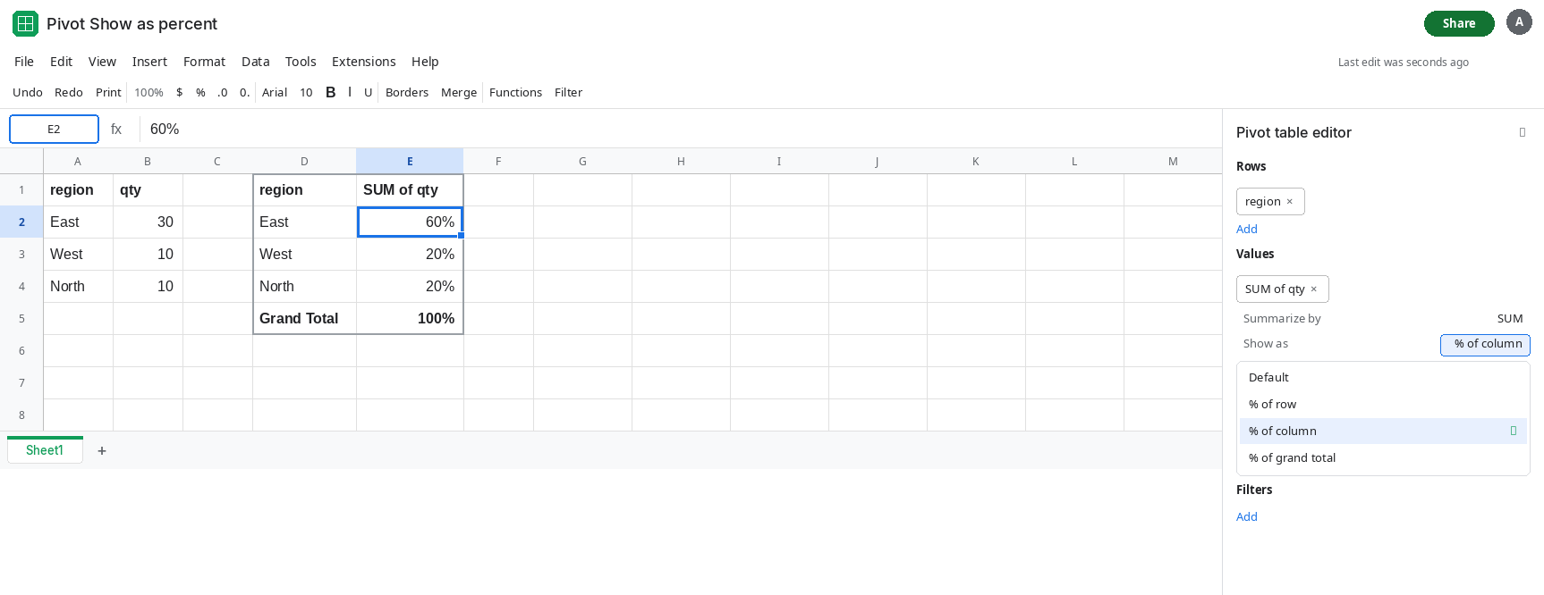
% of row is 100% when the row has one value. Change Show as to % of row. Each region row shows 100%. The row total is that region’s qty, and the row is being compared to itself. The grand total behavior depends on totals, but the region rows are not 60/20/20. This is the “wrong base” report. It is the setting doing what it says. Switch Show as back to % of column so the shares are 60%, 20%, and 20% again.

Re-adding the value drops Show as. In the pivot editor, remove the qty value. The percent column disappears. Add qty again, summarized by SUM. Show as is Default on the new field. The pivot shows 30, 10, and 10. The source is unchanged. The percents did not come back with the field. Leave the pivot on those raw sums. That reset is the bug people hit after they edit the data range or rebuild a value they thought was only summarized by SUM.

A percent format on the source is not Show as. Format B2:B4 as percent. The source displays 3000%, 1000%, and 1000% because 30 formatted as percent is thirty hundred. The pivot, still on Default, follows the numbers 30, 10, and 10, not that format. Put B2:B4 back to automatic or number format so the source reads 30, 10, and 10 again. Do not leave the source formatted as percent.

Leave the pivot showing raw sums after the remove-and-add.

What is actually wrong

• Show as is a display of the aggregated value against a base: the column, the row, or the grand total. Default shows the aggregate itself. Re-adding a value creates a new value field, and the new field starts at Default.
• % of column uses the column total as the base. With one value column, that total is the grand total of qty, and the shares are 60/20/20. % of row uses the row total. With one value in the row, the share is 100%. The base is wrong for “share of the company” even though the menu is working.
• Editing the source range, or a pivot that you recreate because it looked stale, builds values again at Default. The stale-total page is about numbers that do not move when the source changes. This page is about percents that become raw sums after the value field is replaced. See pivot not refreshing.
• A number format on the source column does not set Show as. A number format on the pivot’s value can make 0.6 display as 60% only if the stored pivot value is already the share. Default Show as stores 30. Formatting 30 as percent displays three thousand percent.
• Filters change the base. % of column after you filter out North divides by 40, not by 50. East becomes 75%. That is a new base, not a reset to Default. Read Show as before you call it broken.

This is not the pie chart’s slice-label menu. See pie percent labels. The pivot does not have Slice label.

Fix

Leave the reset pivot on Default so 30, 10, and 10 stay as the broken display.

Set Show as again on the value that exists now. Pivot editor → the qty value → Show as → % of column. East is 60%, West 20%, North 20%. Do this after any remove-and-add. The setting is not stored on the source column, so it does not return by itself.

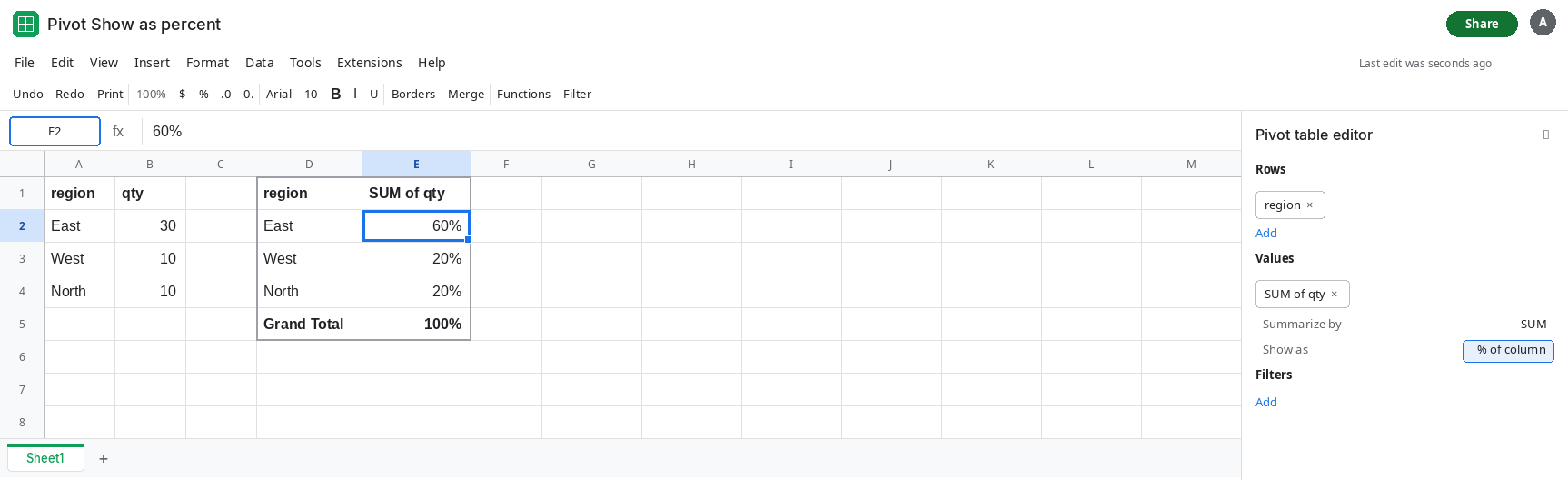
Use % of grand total when you want a share of everything, including across several value columns. % of column is the right base when the column you are reading should total 100%. % of row is the right base when the row should total 100%, which means you need more than one value in the row or the result is trivial.

Or compute the share on the sheet if it must survive a pivot rebuild. =B2/SUM($B$2:$B$4) is 0.6. Format that helper as percent. A pivot that sums a share column will not match % of column, because it will sum 0.6+0.2+0.2. Prefer Show as on the qty, or average the helper only when that is really the question.

If the pivot shows 30 and Show as says Default, the percent mode was cleared when the value was re-added. If every row is 100% and Show as says % of row, the base is the row. If the source format is percent and the formula bar still shows 30, the format is not the pivot setting.