Fix MAXIFS / MINIFS #VALUE! in Google Sheets (mismatched range sizes)

MAXIFS(max_range, criteria_range1, criterion1, …) and MINIFS walk every range in lockstep. A criteria range that is taller or shorter than the max/min range is #VALUE!. The tooltip is Array arguments to MAXIFS are of different size (or MINIFS). Same-size ranges that start on different rows do not always error — they pair by position and can return a quiet wrong max, or 0.

This page is MAXIFS / MINIFS length. It is not COUNTIFS range size (same tooltip family on COUNTIFS/SUMIFS). It is not AVERAGEIF #DIV/0!. It is not FILTER range size (#N/A). Keep the Google Sheets UI in English.

Recreate it on a blank sheet

1. Open a blank spreadsheet. In A1 type region, B1 qty. A2 East. B2 10. A3 West. B3 20. A4 East. B4 5. Three data rows.

MAXIFS — different heights. In D1 type maxifs. In D2 enter =MAXIFS(B2:B4,A2:A5,"East"). B2:B4 is three rows. A2:A5 is four. The cell shows #VALUE!. Tooltip: Array arguments to MAXIFS are of different size. Leave D2 broken.

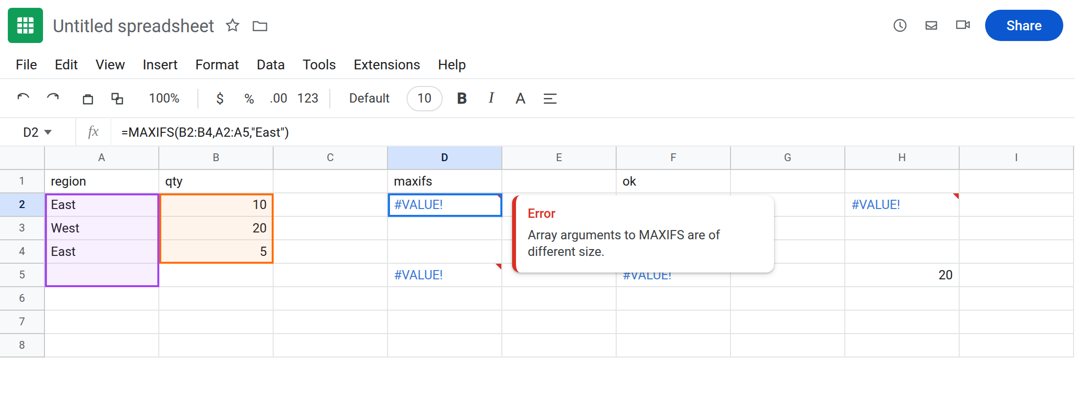
MINIFS — the same mismatch. In D5 enter =MINIFS(B2:B4,A2:A5,"East"). #VALUE!, MINIFS different size. Leave D5 broken.

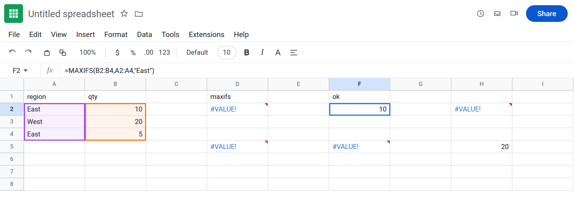
A working MAXIFS. In F1 type ok. In F2 enter =MAXIFS(B2:B4,A2:A4,"East"). The cell shows 10 (East 10 and 5). That row is the control.

Open column vs bounded. In F5 enter =MAXIFS(B2:B,A2:A4,"East"). B2:B to the bottom of the sheet is not the same height as A2:A4. #VALUE!. Leave F5 broken.

COUNTIFS contrast. In H2 enter =COUNTIFS(A2:A4,"East",B2:B5,">0"). #VALUE! on COUNTIFS. Same size story, different function. That primer is COUNTIFS range size. Leave H2 as contrast. Do not copy a COUNTIFS-only memory onto D2 and skip this page — you typed MAXIFS.

Quiet wrong pairing. In H5 enter =MAXIFS(B2:B4,A3:A5,"East"). Both ranges are three rows. No red triangle. A3:A5 is West, East, blank paired with qty 10, 20, 5. The max among “East” in those pairs may be 20 or 5, not the East max 10 you can see in B2:B4. Leave H5 as the silent 3-vs-3 shift.

Leave D2, D5, and F5 broken. Leave F2 as 10.

What is actually wrong

• Every criteria range must match max_range / min_range in row count and column count. Three next to four is #VALUE!.
• B2:B (open) is thousands of rows. A2:A4 is three. Same error as A2:A5.
• Shifted same-height ranges do not error. They zip by position. That is how H5 lies without #VALUE!.
• MAXIFS of no numeric matches is often 0, not #DIV/0!. Empty-average is AVERAGEIF #DIV/0!. Do not debug D2 as “no East.” East is on the sheet.

This is not FILTER #N/A mismatched heights. See FILTER range size.

This is not 10 + pcs. See wrong type. The tooltip names MAXIFS and size.

This is not CHOOSE index 4. See CHOOSE #VALUE!.

Fix

Leave D2, D5, F5, and H2 broken.

Make every range the same rectangle. Keep F2: =MAXIFS(B2:B4,A2:A4,"East"). =MINIFS(B2:B4,A2:A4,"East") is 5. Open columns: =MAXIFS(B2:B,A2:A,"East") — both open — not mixed with A2:A4.

Do not wrap D2 in IFERROR so a size bug prints 0 (which looks like a real min/max). See IFERROR vs IFNA. IFNA will not catch #VALUE!.

If #VALUE! and the tooltip says different size, count rows. If the cell is 0 with matching heights, you have no numeric match (or the criterion missed) — not this #VALUE!. If the number is wrong and heights match, check start rows (H5).

MAXIFS vs COUNTIFS vs AVERAGEIF vs FILTER

MAXIFS/MINIFS size → #VALUE! (D2). This page.

COUNTIFS/SUMIFS size → #VALUE! (COUNTIFS range size). Same sentence, function name in the tooltip.

FILTER size → #N/A (FILTER range size).

AVERAGEIF zero numeric matches → #DIV/0! (AVERAGEIF #DIV/0!). Not a length tooltip. Read the function and the tooltip before you equalize ranges on the wrong page.