Fix RANDARRAY in Google Sheets when the spill is blocked or the values keep changing

RANDARRAY([rows], [columns], [min], [max], [whole_number]) fills a grid with random numbers and spills it from the formula cell. A neighbor inside that rectangle is #REF!. The tooltip names the cell that would be overwritten. rows or columns below 1 is #NUM!. min greater than max is #NUM!. A legal spill has a second trap: RANDARRAY is volatile. It generates new numbers when the sheet recalculates. A VLOOKUP whose key is one of those numbers misses on the next edit even though nobody changed the table.

This page is the blocked spill and the recalc. It is not SEQUENCE spill except that the overwrite tooltip is the same family. It is not SEQUENCE size except that a zero size is #NUM! on both functions. Keep the Google Sheets UI in English.

Recreate it on a blank sheet

1. Open a blank spreadsheet. No source table yet.

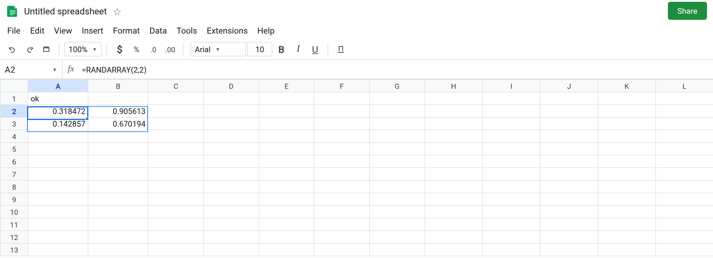
A clear 2×2. In A1 type ok. Leave A2:B3 empty. In A2 enter =RANDARRAY(2,2). Two rows, two columns, decimals between 0 and 1. The four numbers are the control. Write them down. Edit an empty cell, such as D1 (type x, then delete it). A2:B3 changes. The formula did not mention D1. Volatile functions recalculate with the workbook. That is the trap, and the grid is still “working.”

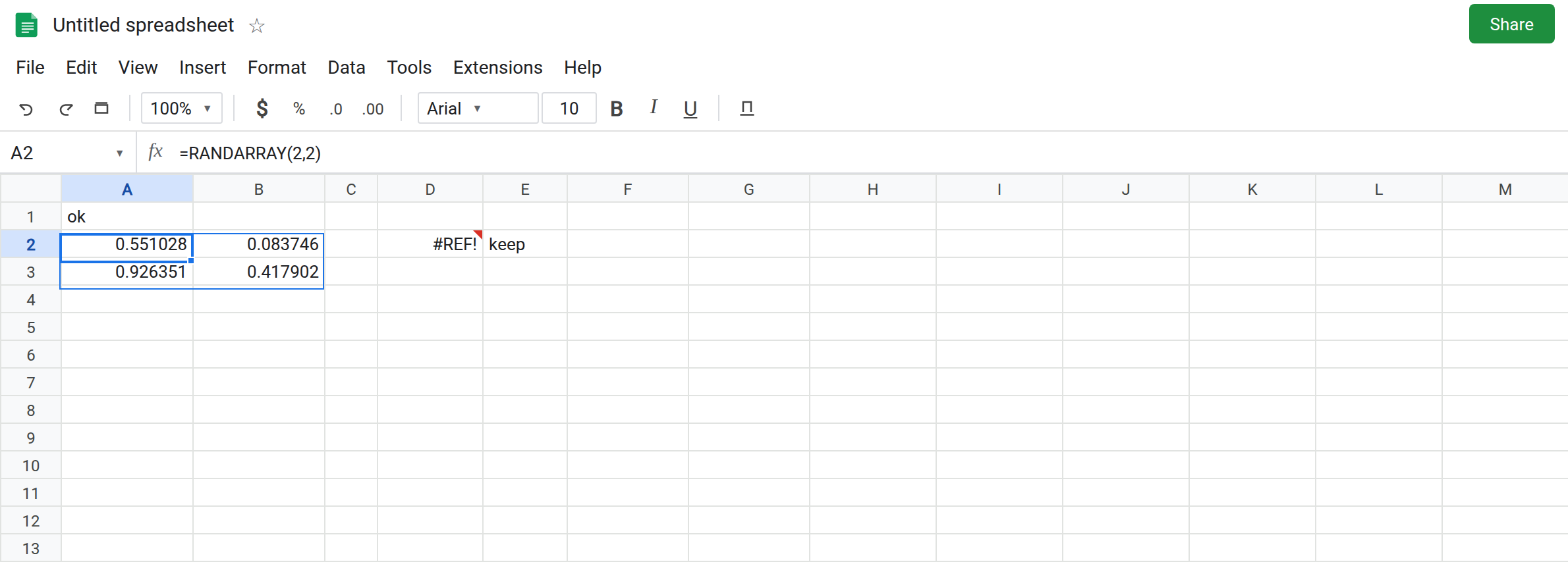
Blocked spill. In E2 type keep. Leave D2 empty. In D2 enter =RANDARRAY(2,2). The rectangle is D2:E3. E2 is occupied. D2 shows #REF!. The tooltip is Array result was not expanded because it would overwrite data in E2. Leave D2 broken. The random function never returned a number there.

Zero rows. In D5 enter =RANDARRAY(0,2). The cell shows #NUM!. Rows must be at least 1, the same rule as SEQUENCE. Leave D5 broken.

Min above max. In D7 enter =RANDARRAY(2,2,10,1). The cell shows #NUM!. The low end is 10 and the high end is 1. Leave D7 broken. Swap them and the call is legal.

Whole numbers. In G1 type ints. Leave G2:G4 empty. In G2 enter =RANDARRAY(3,1,1,6,TRUE). Three integers from 1 through 6. Dice, not decimals. They still change when the sheet recalculates. That column is a second control.

Lookup against a moving key. In I1 type sku, J1 name. I2 1, J2 Widget. I3 2, J3 Gadget. In I5 enter =VLOOKUP(G2,I2:J3,2,FALSE). G2 is one of the dice. Sometimes I5 is a name, sometimes #N/A, because G2 moved and is not 1 or 2. You did not break VLOOKUP. The key is not stable. See VLOOKUP no match only when the key is a value you typed. Leave I5 as whatever it shows after the last calc, and edit D1’s empty neighbor again if you want to watch it flip.

Leave D2, D5, and D7 broken. Leave A2 as a live 2×2.

What is actually wrong

• The spill rectangle is rows by columns starting at the formula. One occupied cell fails the entire call. D2 does not return a partial grid.
• Volatility is separate from #REF!. A2 is not an error. It is a new sample on each calculation. RAND and NOW share that behavior. Now is not this page.
• Using a random cell as an id, a join key, or a QUERY criterion makes the next recalc a different question. I5.
• whole_number TRUE without integer bounds still returns integers inside the range. It does not freeze them.
• min must be less than or equal to max. D7. Equal bounds return that constant, which is legal and still volatile if you leave the formula in place.
• Copying A2 to another cell copies the formula, so you get a second independent sample, not a snapshot of the first.

This is not a circular dependency unless the range arguments include the spill itself (=RANDARRAY(A2) while the formula sits in A2). That #REF! mentions a circular dependency. See circular dependency. D2’s tooltip names E2, not a loop.

Fix

Leave D2, D5, and D7 broken.

Clear the rectangle, then sample. Delete E2 or start the formula where a 2×2 is empty. A2 is already the empty-path version.

Freeze the sample. Select A2:B3, Copy, then Edit → Paste special → Values only, onto A2:B3 or onto a block that does not overlap a formula you still need. The numbers stop changing. The formula is gone. Do this before a lookup. I5 can then use a typed key.

Sizes and bounds. =RANDARRAY(3,1,1,6,TRUE) is G2. Do not pass 0 rows. Do not put the high bound in the min slot.

Do not wrap D2 in IFERROR. You would hide a blocked sample and publish a blank where dice should be. See IFERROR vs IFNA. Do not use RANDARRAY inside IFERROR to “fill misses” on a VLOOKUP column. You would replace missing skus with new random numbers on every edit.

If the tooltip names a cell, clear that cell or move the formula. If the numbers change after an unrelated edit, the formula is still live: paste values. If the tooltip says a size should be at least 1, or the min/max order is wrong, you are in #NUM!, not in a spill block.