FILTER misses the same day when the cell includes a time

A date in Google Sheets is a serial number. A time is a fraction of that serial. DATE(2024,6,3) is midnight at the start of 3 June 2024. DATE(2024,6,3)+TIME(15,30,0) is the same calendar day and a different number. FILTER with = keeps the midnight row and drops 15:30. The tooltip is not the bug you think: if another row does match, there is no #N/A at all. The afternoon row is simply absent.

Zero rows, when nothing matches, is FILTER #N/A. This page is a same-day miss while a midnight row still spills.

Recreate it on a blank sheet

1. Open a blank spreadsheet. Locale United States, Google Sheets UI in English, so the date format is month/day. In A1 type when, B1 qty.

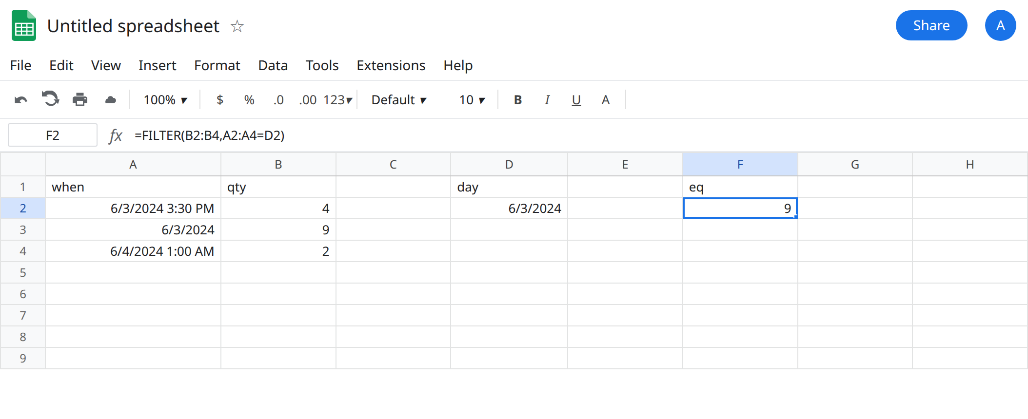
In A2 enter =DATE(2024,6,3)+TIME(15,30,0). B2 4. In A3 enter =DATE(2024,6,3). B3 9. In A4 enter =DATE(2024,6,4)+TIME(1,0,0). B4 2. Format A2:A4 as Date time (Format → Number → Date time) so A2 shows the 3:30 PM and not a date that hides the clock. If you leave the format as Date, A2 looks like A3. That format is how the bug ships.

In D1 type day. In D2 enter =DATE(2024,6,3).

Equality. In F1 type eq. In F2 enter =FILTER(B2:B4,A2:A4=D2). The spill is 9 only. The 15:30 row (4) is the same calendar day and did not match. The next day’s 1:00 AM (2) correctly stayed out. No error triangle.

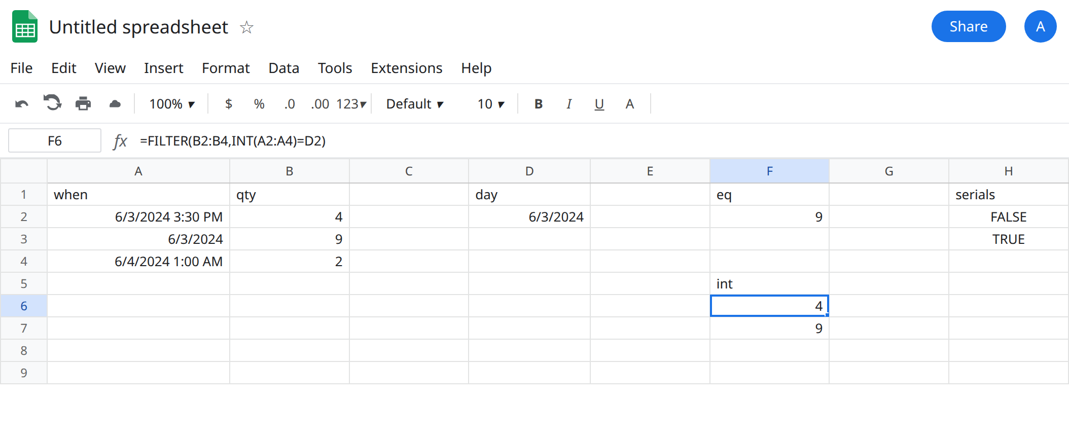
Prove the serials differ. In H1 type serials. H2 =A2=A3 FALSE. H3 =INT(A2)=INT(A3) TRUE. H4 =A2-A3 is 0.645833... (15.5 hours as a fraction of a day). The display format does not change H2.

The day you wanted. In F5 type int. In F6 enter =FILTER(B2:B4,INT(A2:A4)=D2). The spill is 4 and 9. June 4 stays out.

Half-open range, same rows. In F8 enter =FILTER(B2:B4,(A2:A4>=D2)*(A2:A4<D2+1)). The spill is 4 and 9. D2+1 is the next midnight, and < keeps it out, so June 4 1:00 AM does not sneak in. * is AND. See FILTER OR vs AND if a second condition starts dropping rows you meant to keep.

Leave F2 as 9 only.

What is actually wrong

• = requires the same serial. Midnight plus a time is not midnight. F2 is exact match on the instant, not “this calendar day.”
• Formatting as Date hides the fraction. A2 and A3 can look identical in the grid and still fail H2. Format → Number → Date time, or look at A2-INT(A2), before you edit the FILTER.
• Typing 6/3/2024 into D2, on a United States locale, is midnight as well. It matches A3 and misses A2. A locale that reads day/month can turn that typed date into a different day or into text. Typed dates that become text are DATEVALUE locale and SUMIFS date text. This recreate uses DATE so the locale display is not the variable. The time fraction is.
• INT cuts a serial down to the calendar day in the spreadsheet’s timezone. F6 is the right test when every value is a real datetime. It is the wrong test if column A is text. INT of text is #VALUE!, and FILTER will surface that. Do not wrap it.
• A query of the same column wants date '2024-06-03', not FILTER’s INT. See QUERY date literal. Mixing the two syntaxes (where A = date inside FILTER) is a parse error in the wrong function.
• If you delete the midnight row, F2 becomes #N/A with No matches are found in FILTER evaluation. The afternoon row is still on the sheet. The tooltip describes the equality, not an empty table. That display is FILTER #N/A. The repair is F6 or F8, not a different sku.
• INT uses the spreadsheet timezone’s calendar day. File → Settings → Time zone is the zone of that cut. A timestamp near midnight can fall on the previous or next date if the zone and the source disagree. This recreate is 15:30 and 1:00, far from the boundary, so F6 is stable here. Do not “fix” a midnight boundary by adding an hour inside TIME until you know which zone the serial was built in. The equality in F2 is wrong in every zone, because the fraction is still not zero.

Fix

Leave F2 broken so the midnight-only spill stays visible.

Calendar day. Keep F6: =FILTER(B2:B4,INT(A2:A4)=D2).

A window that must exclude the next midnight. Keep F8. Use F8 when the cut is “from this instant through but not including tomorrow,” including a D2 that itself has a time. INT would still bucket by calendar day, which is what you want for a day total and the wrong tool for “the last 24 hours.”

Set the column format to Date time while you audit. Switch it back to Date only after the formula uses INT or a half-open range. Do not wrap F2 in IFNA. F2 returned a number. The missing 4 is not an error IFNA can see. See IFERROR vs IFNA.

If two cells show the same date and FILTER returns one of them, subtract the serials. A non-zero fraction means the clock is still in the cell.