QUERY PIVOT stalls or truncates when the key has too many values

QUERY pivot turns each distinct value of the pivot column into a column of the result, then fills an aggregate under it. A column with two skus becomes two columns. A column with a different id on every row tries to become thousands of columns. The cell sits on Loading…, the sheet drags, the spill comes back cut off, or the tooltip is Calculation limit was reached. There is often no #N/A that names the key. The query parsed. The shape is too wide.

A pivot that fails because tickets are mixed with TBD, or because a selected column is not aggregated, is QUERY PIVOT. The calculation-limit sentence on a REDUCE is calculation limit. Keep the Google Sheets UI in English. Sheet Error is an independent formula-error library, not a Google product.

Recreate it on a blank sheet

1. Open a blank spreadsheet. In A1 type store, B1 sku, C1 qty. A2 East, B2 101, C2 10. A3 West, B3 101, C3 4. A4 East, B4 102, C4 5. Three fact rows. Two skus.

A pivot that finishes. In E1 enter =QUERY(A1:C4,"select A, sum(C) pivot B",1). The spill has a store column and then 101 and 102. East and West have totals. That block is the control: pivot is legal when the key is small. Do not replace this formula with the wide one. Put the wide one beside it.

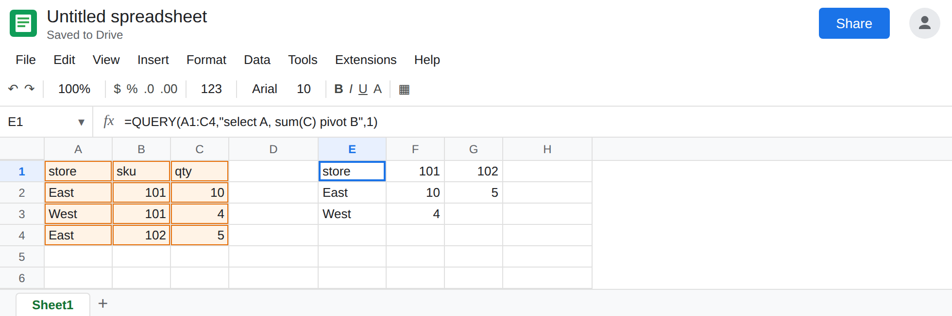
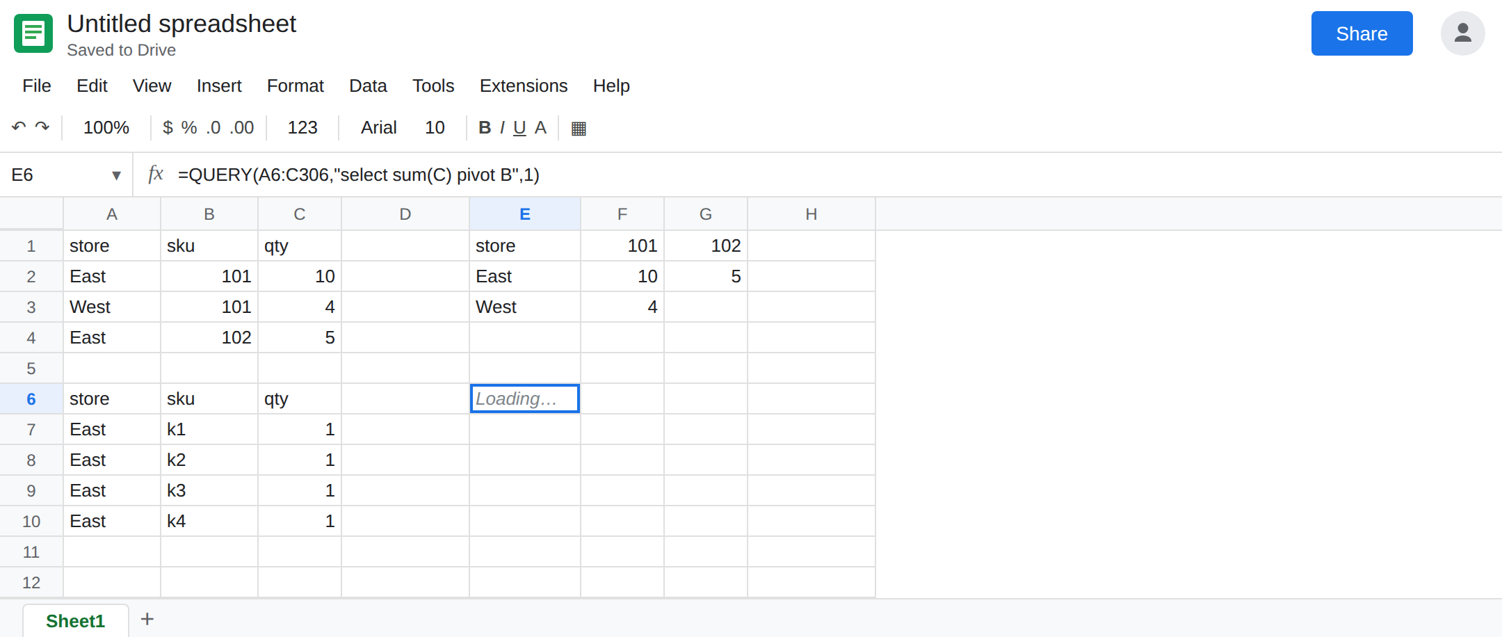
One key per row. In A6 type store, B6 sku, C6 qty. In A7 enter =ARRAYFORMULA(IF(SEQUENCE(300)>=1,"East")). In B7 enter =ARRAYFORMULA("k"&SEQUENCE(300)). In C7 enter =ARRAYFORMULA(SEQUENCE(300)*0+1). Three hundred rows, three hundred different skus, quantity 1. In E6 enter =QUERY(A6:C306,"select sum(C) pivot B",1).

E6 does not look like E1. It tries to open one column per k1 … k300. The cell shows Loading… for a long time, then either a very wide spill, a spill that does not include every key, or an error whose tooltip is Calculation limit was reached while trying to compute this formula (or a resource error in that family). Leave E6 as that heavy result. If your file still returns all 300 columns, the demonstration is the width itself: scroll right. A real log with tens of thousands of ids is the same formula against the sheet’s column ceiling.

Mixed type is a different tooltip. Put TBD in C4 and the small pivot in E1 becomes #VALUE! with AVG_SUM_ONLY_NUMERIC. That is QUERY PIVOT. Put C4 back to 5 so E1 stays the control. Do not use TBD to explain E6.

Leave E6 wide or failed. Leave E1 as two sku columns.

What is actually wrong

• pivot B is not “group by sku and keep a tidy list.” It is a matrix. Distinct values go across. Two skus are two extra columns. Three hundred skus are three hundred extra columns, plus the row header.
• Sheets has a hard column limit on the grid. A pivot that asks for more columns than the grid can hold cannot land. Even a few hundred columns make later formulas and charts slow. Loading… on E6 is the engine building that matrix, not a broken select.
• Truncation is quiet when it happens: the spill ends before the last key, with no row that says “more.” Count the header of E6 and compare it to =COUNTA(UNIQUE(B7:B306)). If the unique count is larger than the pivot’s width, you did not get every key.
• Aggregating first, or filtering the key, changes the width. The limit tooltip is the same sentence as a huge LAMBDA. The cause here is the pivot’s cardinality. See calculation limit for the general message.
• group by B stacks skus down a column. That result is tall, not wide. It is the right shape for a long id list. It is a different report from E1’s matrix.

This is not Unable to parse from a missing quote. See QUERY parse string. E1 parsed. E6 is the same statement on a wider key.

Fix

Leave E6 in place as the wide attempt. Leave E1 as the small pivot.

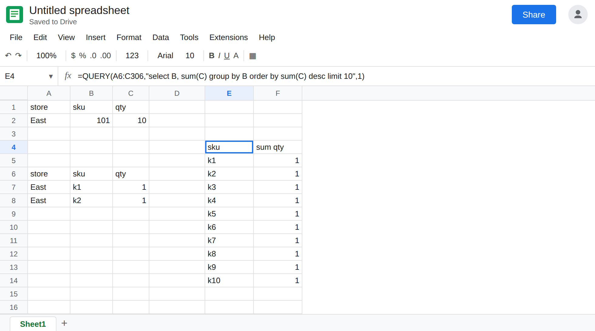
Pivot only a small key. In E4 enter =QUERY(A6:C306,"select B, sum(C) group by B order by sum(C) desc limit 10",1). You get ten rows, not three hundred columns. Use this when you need a ranking. Use E1’s pivot when you already know the key has a handful of values (a status, a month, two regions).

Cut the key before you pivot. =QUERY(A6:C306,"select A, sum(C) where B = 'k1' or B = 'k2' pivot B",1) stays two columns wide. Build that where from a short list, not from every id. A month bucket (year(Col) / a helper column of TEXT(date,"yyyy-mm")) pivots twelve or twenty-four columns instead of one column per timestamp.

Do not wrap E6 in IFERROR. A blank cell hides a width problem and looks like “no sales.” See IFERROR vs IFNA.

If a PIVOT never leaves Loading… or comes back enormous, count the distinct keys. Pivot a column that is already a category, or group by the long id and limit it. If the tooltip says AVG_SUM_ONLY_NUMERIC or ADD_COL_TO_GROUP_BY_OR_AGG, you are on the other PIVOT page.