XLOOKUP spills the return array across when you expected the months stacked down

XLOOKUP returns the slice of return_array that lines up with the match. If the lookup range is a column and the return range is several columns wide, the hit spills across. If the lookup range is a row and the return range is several rows tall, the hit spills down. The function is not choosing the direction you had in mind. It is using the direction you passed. A clear sheet shows the values. The surprise is the shape.

A two-column return that cannot spill because the next cell is filled is XLOOKUP return spill. This page leaves the path empty and gets the wrong orientation. Keep the Google Sheets UI in English. Sheet Error is an independent formula-error library, not a Google product.

Recreate it on a blank sheet

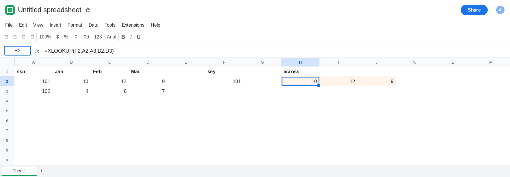
1. Open a blank spreadsheet. In A1 type sku, B1 Jan, C1 Feb, D1 Mar. A2 101, B2 10, C2 12, D2 9. A3 102, B3 4, C3 8, D3 7. Sku 101 is Jan 10, Feb 12, Mar 9.

A column lookup and a wide return spill across. In F1 type key. F2 101. Leave H2:J2 empty. In H1 type across. In H2 enter =XLOOKUP(F2,A2:A3,B2:D3). The spill is one row and three columns: 10, 12, 9 in H2:J2. Nothing is stacked under H2. The months are the width of B2:D3. That row is the shape people often wanted as a column. Leave H2 as the horizontal spill.

A row lookup and a tall return spill down. In F4 type month. F5 Feb. Leave H5:H6 empty. In H4 type down. In H5 enter =XLOOKUP(F5,B1:D1,B2:D3). The lookup range is the header row, three columns. The return range is two rows tall and three columns wide, so the heights match on the search axis. The spill is 12 in H5 and 8 in H6. Feb’s two skus, stacked. It does not spill into I5. Leave H5 as that column.

A one-row return against a two-row lookup. In H8 enter =XLOOKUP(F2,A2:A3,B2:D2). A2:A3 is two rows. B2:D2 is one row. The cell errors (#N/A / #VALUE!). The return range has to share the lookup’s height when the lookup is vertical. Wanting a row is not a reason to pass a shorter one. Leave H8 broken.

One cell, so you can see a single month. In H10 enter =XLOOKUP(F2,A2:A3,C2:C3). The cell shows 12. Feb only. A value in I10 would not matter. The wide spill is H2, not this cell.

Leave H2 horizontal. Leave H5 vertical. Leave H8 broken.

What is actually wrong

• Orientation is the extra dimension of return_array. Vertical lookup plus a 2×3 return yields 1×3. Horizontal lookup plus a 2×3 return yields 2×1. H2 and H5 are those two results from ranges that are legal.
• B2:D2 looks like “the three months for one sku,” and it is, but only if the lookup range is also one row tall. Against A2:A3 it is a size error. H8. The working horizontal spill includes both skus’ rows in the return range and lets XLOOKUP pick the row.
• TRANSPOSE flips a legal spill. It does not repair H8. Transpose after H2, not instead of a matching range.
• An occupied cell in the spill path is #REF! with the overwrite tooltip. I2 empty is why H2 can show 12. If I2 had text, you would be on XLOOKUP return spill.
• Binary search and last-match do not change the shape. They change which row is chosen. See XLOOKUP binary search.

Fix

Leave H2 as the sideways months. Leave H8 broken.

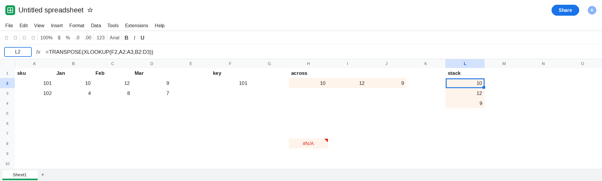
Stack the months. In L1 type stack. Leave L2:L4 empty. In L2 enter =TRANSPOSE(XLOOKUP(F2,A2:A3,B2:D3)). L2:L4 is 10, 12, 9 downward. The XLOOKUP is the same call as H2. TRANSPOSE is the whole difference.

Return a column when you only need one month. Keep H10 for Feb. Narrow return_array to C2:C3 instead of transposing a row you did not want.

Match the search axis before you worry about direction. A vertical lookup needs a return range with the same number of rows. A horizontal lookup needs a return range with the same number of columns. H5 is the horizontal-lookup pattern: headers in B1:D1, body in B2:D3.

Do not wrap H8 in IFERROR. The sizes disagree. See IFERROR vs IFNA.

If the months appear to the right of the formula, return_array is wider than one column. TRANSPOSE that spill when the report needs a column. If the formula errors and the return range is a single row while the lookup range is several rows, give the return range the same height first.