

CORREL returns #DIV/0! when one column does not vary
Updated
CORREL(range1, range2) returns the Pearson correlation of the paired numbers. The formula divides by the product of the two standard deviations. If every value in one range is the same number, that standard deviation is 0, and the division is #DIV/0!. The other column can be a perfect ramp. The pairs can be complete. The correlation is undefined, not “no relationship.” A correlation of 0 means the two columns vary and do not move together linearly. Replacing #DIV/0! with 0 reports a relationship you did not measure.
A plain division by an empty cell is divide by zero. STDEV of a constant is the zero in the denominator. Keep the Google Sheets UI in English. Sheet Error is an independent formula-error library, not a Google product.
Recreate it on a blank sheet
Section titled “Recreate it on a blank sheet”- Open a blank spreadsheet. In A1 type
x, B1y. A21, B22. A32, B34. A43, B46. A54, B58. Four pairs on the line y = 2x.
A correlation that exists. In D1 type ok. In D2 enter =CORREL(A2:A5,B2:B5). D2 is 1. The columns move together perfectly. =STDEV(A2:A5) is not 0. =STDEV(B2:B5) is not 0. That cell is the control.
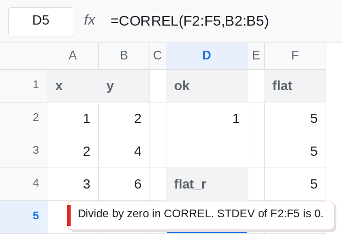
One column is constant. In F1 type flat. F2 5. F3 5. F4 5. F5 5. In D4 type flat_r. In D5 enter =CORREL(F2:F5,B2:B5). D5 is #DIV/0!. Column F does not vary. Column B varies. The tooltip is a divide-by-zero inside the correlation, not a complaint that B failed. =STDEV(F2:F5) is 0. =STDEV.S(F2:F5) is 0. Leave D5 broken.
Both columns constant. In H2 type 5 and fill H2:H5 with 5. In D7 enter =CORREL(F2:F5,H2:H5). D7 is #DIV/0! as well. Two flat columns are not “perfectly correlated.” There is no line to fit. Leave D7 broken.
Too few numeric pairs. In A6 type note. In B6 type 10. In D9 enter =CORREL(A2:A6,B2:B6). A6 is text. CORREL ignores that pair. The numeric pairs are still the original four, so D9 is 1. Now restrict the ranges to a single pair: in D11 enter =CORREL(A2:A3,F2:F3). F2:F3 is 5 and 5. Still constant, #DIV/0!. In D13 enter =CORREL(A2,B2). One cell against one cell is not two pairs. D13 is #DIV/0! or #N/A depending on the build; either way it is not a correlation you can publish. You need at least two numeric pairs, and those pairs need variation in both columns. Leave D5 as the clear constant-column case.
A real zero is not this error. In J2 1. J3 2. J4 3. J5 4. In K2 1. K3 1. K4 2. K5 2. The x values vary. The y values vary. They are not a straight line through the origin of a perfect correlation, and they are not constant. In D15 enter =CORREL(J2:J5,K2:K5). D15 is a number, not #DIV/0!. On these points it is about 0.894. It is not 0. The point of the cell is the token: a computed correlation is a number. D5 is an error. Do not round D5 into 0 and call it D15.
Leave D5 and D7 as #DIV/0!. Leave D2 as 1.
What is actually wrong
Section titled “What is actually wrong”- The denominator is the two standard deviations. Either one being
0is#DIV/0!. F2:F5. The other range can be perfectly numeric. CORRELignores text and blanks, then uses the pairs that remain. If ignoring text leaves one column constant, or leaves fewer than two pairs, you get the same#DIV/0!as a column that was typed as constants. A helper that returns=""can strip the variation out. See COUNTUNIQUE blanks for how formula blanks pretend to be empty. Here they pretend a column still has numbers.#N/Ainside either range makesCORRELreturn#N/A, which is not D5. Catch that in the source if you meant to drop the pair. See IFNA vs IFERROR spill.- A result of
0would mean “we measured no linear relationship.” D5 was not measured.IFERROR(D5,0)publishes the wrong sentence. PEARSONis the same calculation and the same#DIV/0!on a constant column. Renaming the function does not invent a variance.
This is not divide by zero from =B2/A2 with A2 empty. The formula in D5 is CORREL. The zero is inside the function, and STDEV of F2:F5 shows it.
Leave D5 broken. Leave D2 as 1.
Do not correlate a constant. If =STDEV(F2:F5)=0, stop. The column is flat. Find the input that was supposed to vary: a copied-down default, a rounded series that became one value, or text that CORREL skipped until one number remained. Fix that column. Then =CORREL(F2:F5,B2:B5) can return a number.
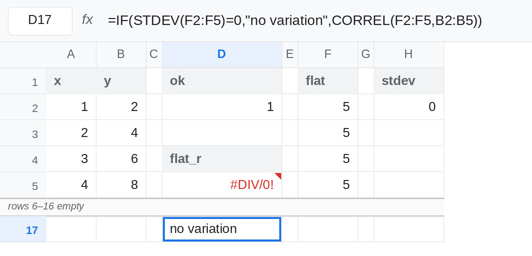
Say “undefined” when the sheet must stay filled. In D17 enter =IF(STDEV(F2:F5)=0,"no variation",CORREL(F2:F5,B2:B5)). D17 is no variation. The same test belongs on the other column if either side might be flat: =IF(OR(STDEV(F2:F5)=0,STDEV(B2:B5)=0),"no variation",CORREL(F2:F5,B2:B5)). Do not return 0 from the IF. A later average of correlations would treat “undefined” as “uncorrelated.”
Two pairs, both moving, is the minimum shape. D2’s four points are enough. One point is not. Two points that differ in both columns return 1 or -1, which is a real result on a tiny sample, not a #DIV/0!. If that 1 looks too sure, you need more rows, not IFERROR.
If the tooltip is divide by zero and STDEV of one range is 0, the correlation is undefined. If STDEV of both ranges is positive and the cell is #N/A, a pair contains #N/A. If the cell is a number, including 0, the function finished. Leave that 0 alone.