A slicer does nothing when its range is not the pivot source

A slicer is a filter control on the sheet. It filters pivot tables and charts whose data range is the same range the slicer uses. Insert → Slicer on a second copy of the numbers does not talk to a pivot that still reads the first copy. You can click West all day. The pivot keeps East and West. The slicer is not broken. It is connected to a different rectangle.

A pivot that ignores a new row under its range is pivot not refreshing. GETPIVOTDATA is GETPIVOTDATA. A QUERY pivot clause is QUERY PIVOT. Keep the Google Sheets UI in English. Sheet Error is an independent formula-error library, not a Google product.

Recreate it on a blank sheet

1. Open a blank spreadsheet. In A1 type store, B1 qty. A2 East, B2 10. A3 West, B3 4. A4 East, B4 6. East’s total is 16. West’s is 4.

A pivot on A1:B4. Select A1:B4. Insert → Pivot table. Put it on the same sheet, starting at D1, or on a new sheet if you prefer. Rows: store. Values: qty summarized by SUM. The pivot shows East 16 and West 4. The editor’s range is Sheet1!A1:B4 (quotes around the sheet name if the UI adds them). That pivot is the control.

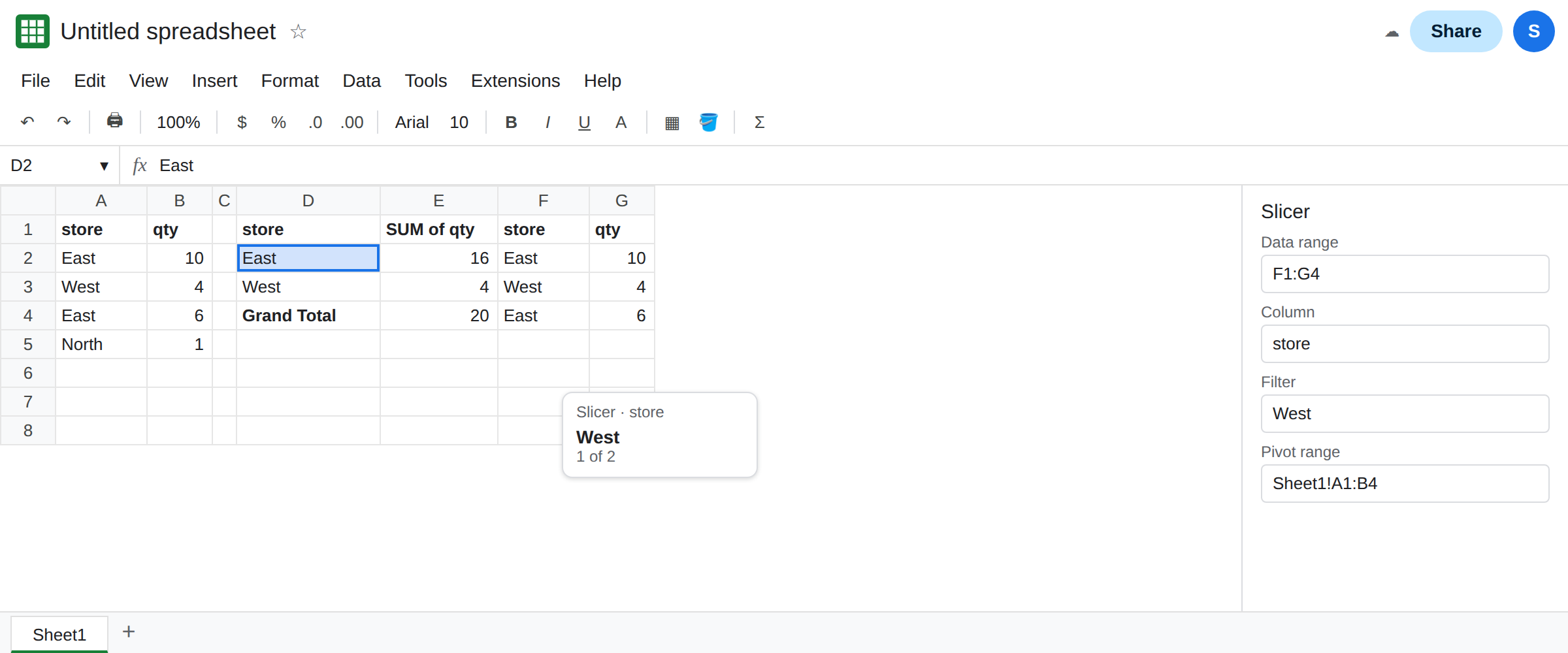
A copy of the data, and a slicer on the copy. Select A1:B4, copy, and paste at F1. F1:G4 matches A1:B4. Click a blank cell. Insert → Slicer. In the slicer panel, set the data range to F1:G4 if it did not guess that. Set the column to store. The slicer appears on the sheet. Open it and leave only West checked. Column F’s visible filter may change if the slicer is acting on that range. Look at the pivot. East is still 16 and West is still 4. The slicer did not edit D1’s pivot. Leave West as the only slicer choice and leave the pivot showing both stores.

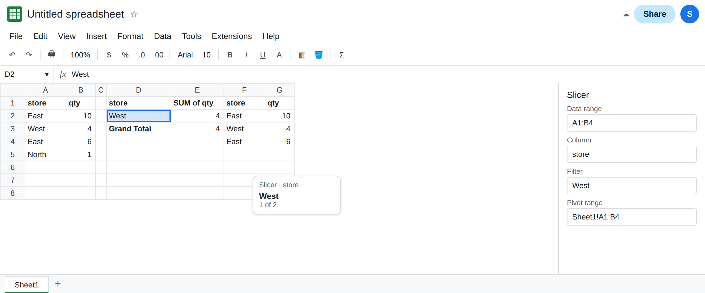
The same range connects them. Edit the slicer. Set its data range to A1:B4, column store. Filter to West only. The pivot shows West 4 and drops East, or East’s sum disappears from the pivot, because the slicer is now on the pivot’s source. Clear the slicer (select all stores). East 16 and West 4 return. That is the control for a connected slicer. Set the slicer range back to F1:G4 and filter to West again so the disconnected state is what you leave on the sheet for the lesson, after you have seen the pivot move once.

A chart built on F1:G4 is a different object. A chart of the copy follows the slicer that points at the copy. The pivot still does not. “The slicer works” and “the pivot changed” are two tests. This page fails the second test on purpose.

A filter view on A1:B4 is not a slicer. See filter view vs filter.

What is actually wrong

• The slicer stores a range and a column. The pivot stores a range. They filter each other when those ranges are the same. F1:G4 and A1:B4 are two sources that happen to contain the same words.
• Clicking the slicer does not refresh a pivot cache and does not widen a pivot range. If the pivot is stale because row 5 is outside A1:B4, that is pivot not refreshing. A connected slicer will not add row 5 either.
• The column name has to exist on that range. A slicer set to store while the range’s header says shop has nothing to filter. Rename with the header, then pick the column again.
• More than one pivot on A1:B4 will all follow a slicer on A1:B4. A pivot on another tab that uses 'Sheet1'!A1:B4 is the same range. A pivot that uses a different tab’s copy is not.
• GETPIVOTDATA reads whatever the pivot currently shows. It does not attach a slicer. A #REF! from that function is GETPIVOTDATA.

This is not Insert → Chart with a filter icon on a header. That icon is a sheet filter or a chart filter, and it is a different control from a slicer object.

Fix

Leave one slicer on F1:G4 filtered to West, with the pivot still showing East 16, so the disconnect stays visible. Add a second slicer for the fix, or repoint the first after you have compared them.

Set the slicer range to the pivot range. Select the slicer. In the panel, data range A1:B4, column store. Filter to West. The pivot’s East row drops. Select all stores in the slicer and both totals return.

When you meant to filter the copy, point the pivot at the copy. Change the pivot’s range to F1:G4 in the Pivot table editor. Then a slicer on F1:G4 moves those totals. Do not maintain two rectangles unless two reports are what you want.

Do not rebuild the pivot with SUMIF to imitate a slicer. The slicer already filters a pivot that shares its range.

If the slicer changes and the pivot does not, read both range boxes. They are different rectangles. If they match and a new row is missing, the range ends above that row. That is the pivot page, not a disconnected slicer.