Fix QUERY #VALUE! in Google Sheets (dates mixed with text)

Some cells in column A look like dates and QUERY still returns #VALUE!. The formula is not reading the dates you can see. It is reading the whole column’s type. One text cell (TBD, unknown, pending) is enough to stop year(A).

Recreate it on a blank sheet

1. Open a blank spreadsheet. Leave the tab named Sheet1. In A1 type date, B1 item.
2. In A2 type 2024/1/15 so Sheets stores a real date. B2 Widget. A3 TBD as plain text. B3 Skip. A4 2/1/2024 as a real date. B4 Gadget. A5 unknown. B5 Thing. A6 pending. B6 Doohickey.
3. In D1 enter exactly =QUERY(A1:B6,"select year(A), B",1). The cell shows #VALUE!. The tooltip is Unable to parse query string for Function QUERY parameter 2: Can’t perform the function year on a column that is not a Date or a DateTime column.

D1 selected. Formula bar shows =QUERY(A1,"select year(A), B",1). D1 is #VALUE!. Tooltip says year cannot run on a column that is not a Date or a DateTime column.

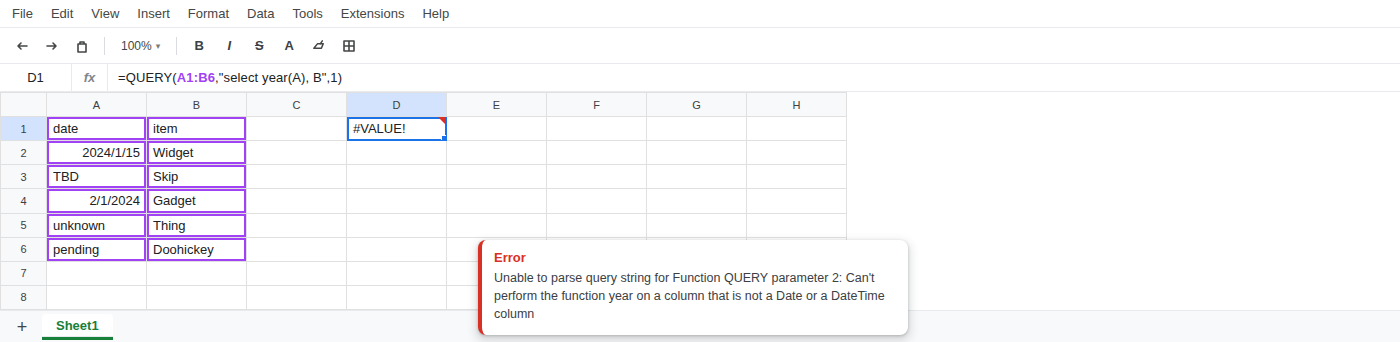
Leave D1 as the broken formula.

where A > date '2024-01-01' is not this recreate. On a short table that filter can succeed and hide the mixed-type problem. The recreate is year(A) on the mixed A column.

Second recreate — month() on the same mix. In D4 enter =QUERY(A1:B6,"select month(A), B",1). The cell shows #VALUE!. Same tooltip family. month, day, quarter, and year all require a Date or DateTime column. The text cells in A are enough. Leave D4 broken.

In F1 type is_date. In F2 enter =ISNUMBER(A2). TRUE (Sheets stores dates as numbers). In F3 enter =ISNUMBER(A3). FALSE. That pair is the mix. You do not need QUERY to see it.

What is actually wrong

QUERY inspects a whole column’s type. Column A mixes real dates with text (TBD, unknown, pending). That mix is not a Date or DateTime column. year(A) only runs on a Date or DateTime column. Mixed type is why the query string fails to parse. The dates you can see in A2 and A4 are not ignored. They are in a column QUERY has already typed as mixed / not-date.

This is not a locale / comma-vs-semicolon parse error. That is #ERROR! with Formula parse error from argument separators. See locale parse error. D1 used commas inside a quoted query string. The Sheets formula parsed. QUERY then rejected the statement.

This is not IMPORTRANGE select A vs Col1. That page is often #N/A on an import array. See Col1 vs A. D1 is a sheet range. A is the correct letter. The column is the wrong type.

This is not the other Unable to parse query string recreates (unquoted Widget, a bare 2024-01-01 without date '...'). Those live on QUERY parse string. Read the tooltip. This one names year and Date / DateTime.

This is not #VALUE! from 10 + pcs. See wrong type. Nothing is being added. This is not FILTER #N/A. See FILTER no match.

Fix

Do not QUERY the mixed column.

Leave D1 and D4 as the broken formulas so #VALUE! stays on the sheet.

Helper column: C1 date_clean. In C2 enter =IF(ISNUMBER(A2),A2,"") and fill down through C6. Text cells become blank. Real dates remain.

Then in E1 enter =QUERY({C1:C4,B1:B4},"select Col1, Col2 where Col1 > date '2024-01-01'",1). The formula spills headers plus the two date rows: Widget and Gadget.

E1 selected. Formula bar shows =QUERY({C1,B1},"select Col1, Col2 where Col1 > date '2024-01-01'",1). Spill is date_clean / item with Widget and Gadget. Column C shows cleaned dates and blanks. D1 is still #VALUE!.

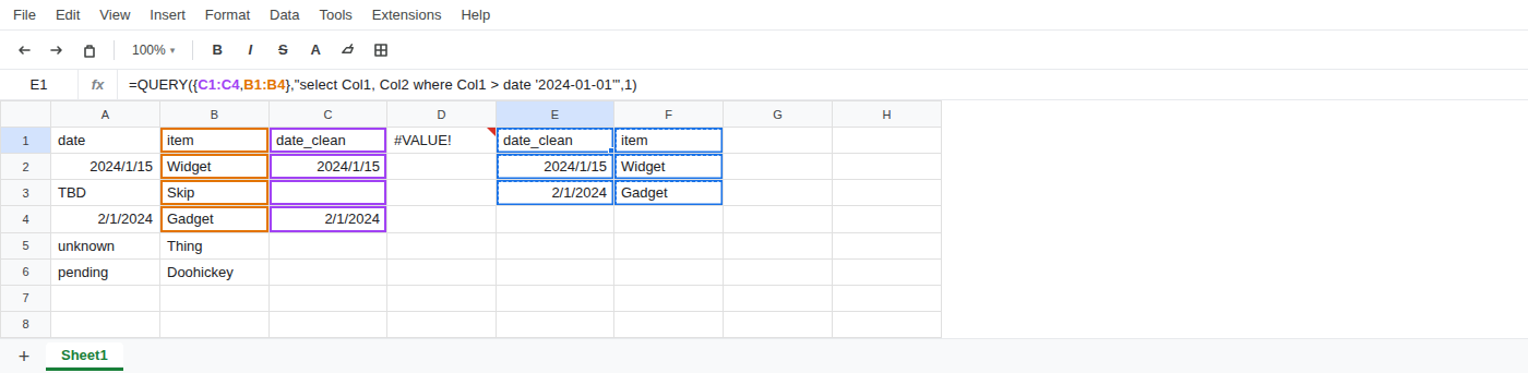
The helper is wrapped in { }, so the query uses Col1 and Col2, not A and B. That switch is expected. It is not the bug on this page.

You can year() the cleaned column the same way: =QUERY({C1:C6,B1:B6},"select year(Col1), Col2 where Col1 is not null",1) after the helper is filled through C6. Do not put year(A) back on A1:B6 until A has no leftover text.

Do not wrap this in IMPORTRANGE. Do not change File > Settings locale. Do not try to make the mixed column one QUERY without the helper. Do not wrap D1 in IFERROR until the column is actually dates — that only hides the type mix.

If year fails on a column that looks like dates, look for leftover text in that column first.