AVERAGEIFS returns #VALUE! when the ranges are different sizes

AVERAGEIFS(average_range, criteria_range1, criterion1, …) averages numbers whose rows pass every test. The average range and every criteria range have to be the same size. One extra row is #VALUE!. The tooltip is Array arguments to AVERAGEIFS are of different size. When the sizes match and no numeric cell passes, the result is #DIV/0!, the same family as AVERAGEIF with nothing to average. Those are different failures. Resizing will not fix a real empty group, and a guard for #DIV/0! will not fix a taller range.

AVERAGEIF with one criterion and zero numeric matches is AVERAGEIF #DIV/0!. COUNTIFS / SUMIFS size is COUNTIFS range size. MAXIFS size is MAXIFS / MINIFS size. Keep the Google Sheets UI in English. Sheet Error is an independent formula-error library, not a Google product.

Recreate it on a blank sheet

1. Open a blank spreadsheet. In A1 type region, B1 qty. A2 East, B2 10. A3 West, B3 20. A4 East, B4 30. A5 North, B5 40. Four data rows.

A working average. In D1 type ok. In D2 enter =AVERAGEIFS(B2:B5,A2:A5,"East"). The average range is first. East is 10 and 30. D2 is 20. That cell is the control.

Criteria range one row taller. In D4 type tall. In D5 enter =AVERAGEIFS(B2:B5,A2:A6,"East"). B2:B5 is four rows. A2:A6 is five. The cell shows #VALUE!. Tooltip: Array arguments to AVERAGEIFS are of different size. A6 is blank. A blank extra row still counts as a row. Leave D5 broken.

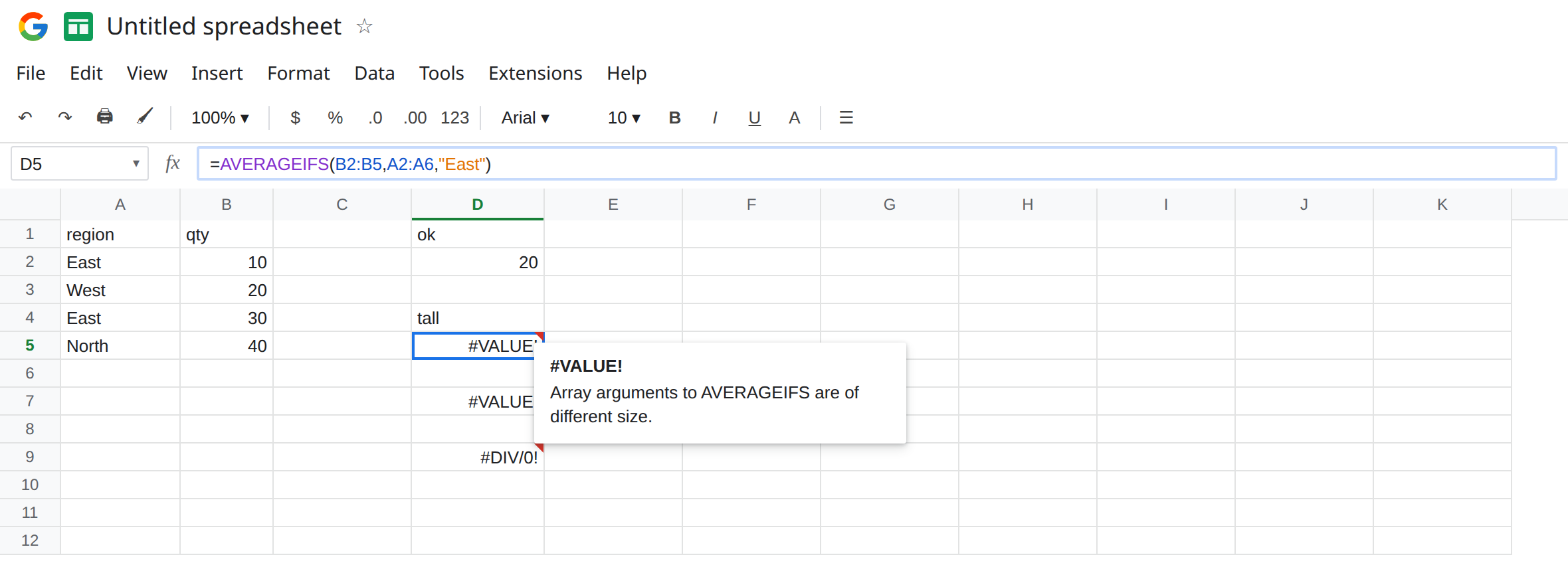
Open average range, closed criteria. In D7 enter =AVERAGEIFS(B2:B,A2:A5,"East"). B2:B is the rest of the column. #VALUE!. Leave D7 broken.

No match, sizes equal. In D9 enter =AVERAGEIFS(B2:B5,A2:A5,"South"). Shapes match. South is not on the sheet. The cell shows #DIV/0!. There is nothing to divide the sum by. This is not the size tooltip. Leave D9 as #DIV/0!.

Text in the average range. In B6 type TBD and widen nothing. Do not point D2 at B6. In F2 enter =AVERAGEIFS(B2:B6,A2:A5,"East"). Five numbers-and-text versus four regions. #VALUE! again, because the heights differ, before Sheets ever decides what to do with TBD. If you extend the region too — A6 blank, ranges B2:B6 and A2:A6 — the size error goes away and East is still 20. TBD is not East, so it never enters the average. A text cell inside a matched East row is ignored by the average the way AVERAGE ignores text, or it can produce #DIV/0! if it was the only East cell. The size tooltip is the one in D5. Do not debug TBD while D5 is still #VALUE!.

Argument order. AVERAGEIFS puts the range you average first. =AVERAGEIFS(A2:A5,"East",B2:B5) is the SUMIFS habit (criteria before the values) applied to the wrong function. That call is #VALUE! for a different reason: a criterion sitting where a range should be, or ranges that no longer pair. Leave a scratch cell F5 with that formula if you want to see it fail. The repair is D2’s order, not a longer range.

Leave D5, D7, and D9 broken in their two different ways. Leave D2 as 20.

What is actually wrong

• average_range sets the shape. Every criteria_range must match it in rows and in columns. Four next to five is #VALUE!.
• The tooltip names AVERAGEIFS and “different size.” A #DIV/0! with no size sentence is D9: the filter kept zero numbers. South is that case. East is not.
• Open-ended columns are large. B2:B with A2:A is matched. B2:B with A2:A5 is D7.
• Same size, different start row, does not throw. =AVERAGEIFS(B2:B5,A3:A6,"East") pairs B2 with A3. You can get 30, or 20, or #DIV/0!, with no size tooltip. If D2 is 20 and a shifted copy is not, look at the start row.
• Two criteria still share one shape. A status in C2:C5 is =AVERAGEIFS(B2:B5,A2:A5,"East",C2:C5,"open"). C2:C6 brings the tooltip back.
• AVERAGEIF (no S) takes the criterion range first and the average range second, the opposite of AVERAGEIFS. Swapping those names is how F5 happens. This page’s D5 is height, with the arguments already in AVERAGEIFS order.

This is not 10 + pcs. See wrong type. D5 parsed, then rejected the shapes.

This is not FILTER #N/A for a short condition. See FILTER range size.

Fix

Leave D5, D7, and D9 on the sheet.

Match the rectangles. Keep D2. In E2 enter =AVERAGEIFS(B2:B,A2:A,"East"). E2 is 20. Both ends open.

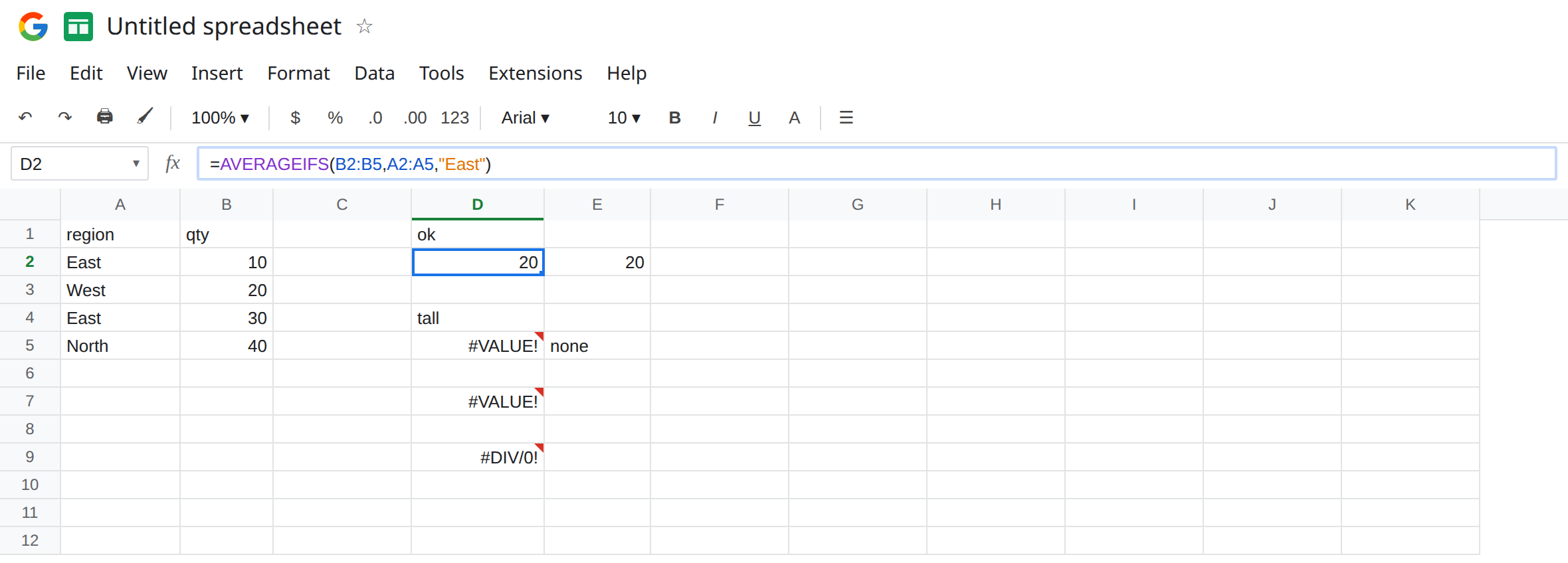
Guard the empty group, not the size bug. In E5 enter =IF(COUNTIFS(A2:A5,"South")=0,"none",AVERAGEIFS(B2:B5,A2:A5,"South")). E5 is none. The COUNTIFS ranges are the same height as each other. This guard is for D9. It does not make D5 a number. If you put the guard on D5, COUNTIFS of mismatched ranges is itself #VALUE!, and IF will not save it.

Do not wrap D5 in IFERROR(...,0). An average of 0 and a broken shape would look alike, and East is 20, not 0. See IFERROR vs IFNA.

If the tooltip says different size, count rows in the average range and in each criteria range. If the cell is #DIV/0! and the tooltip does not mention size, the shapes match and no number passed (D9). If the average is a quiet wrong number, check the start row and check that you did not average the region column.

#VALUE! vs #DIV/0!

D5 and D7 are size #VALUE! (this page). D9 is #DIV/0! on a legal shape, the same idea as AVERAGEIF #DIV/0!. D2 is 20. Read the tooltip before you add rows, and read #DIV/0! before you delete the criterion.