BYROW errors when the LAMBDA returns two columns with HSTACK

BYROW runs a LAMBDA once per row and must get one value back. HSTACK(SUM(row),AVERAGE(row)) is two values. So is {SUM(row),AVERAGE(row)}. The cell is #N/A or #VALUE!. The tooltip is Single value expected. Nested array results are not supported. The hours are numbers. The return shape is the bug.

A lambda that returns the row itself is BYROW / MAP LAMBDA. This page is the two-metric return: sum and average, built with HSTACK or an array literal. HSTACK of two finished BYROW spills is legal, because each BYROW already returned one column. Keep the Google Sheets UI in English. Helper names stay English: LAMBDA, BYROW, HSTACK.

Recreate it on a blank sheet

1. Open a blank spreadsheet. In A1 type mon, B1 tue, C1 wed. A2 2, B2 2, C2 1. A3 0, B3 4, C3 3. A4 5, B4 1, C4 1. Three days, three rows. Row totals are 5, 7, 7. Row averages are 5/3, 7/3, 7/3.

One number per row. In E1 type sum_only. In E2 enter =BYROW(A2:C4,LAMBDA(row,SUM(row))). E2:E4 is 5, 7, 7. That column is the control. One scalar each time.

HSTACK inside the lambda. In E6 type hstack_in. In E7 enter =BYROW(A2:C4,LAMBDA(row,HSTACK(SUM(row),AVERAGE(row)))). The cell shows #N/A or #VALUE!. Tooltip: Single value expected. Nested array results are not supported. HSTACK asked each row’s result to be two cells wide. BYROW will not spill a table of rows. Leave E7 broken.

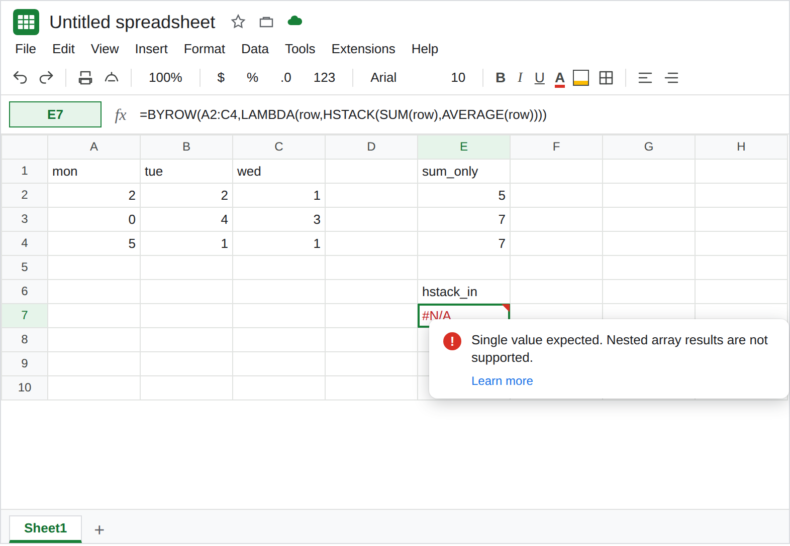
The curly form is the same refusal. In E9 enter =BYROW(A2:C4,LAMBDA(row,{SUM(row),AVERAGE(row)})). Same tooltip. {sum, average} is two cells. Leave E9 broken. If { is Formula parse error before BYROW runs, the array separator for your locale is not a comma. See array literal locale. Fix the separator, and E9 is still the nested-array error.

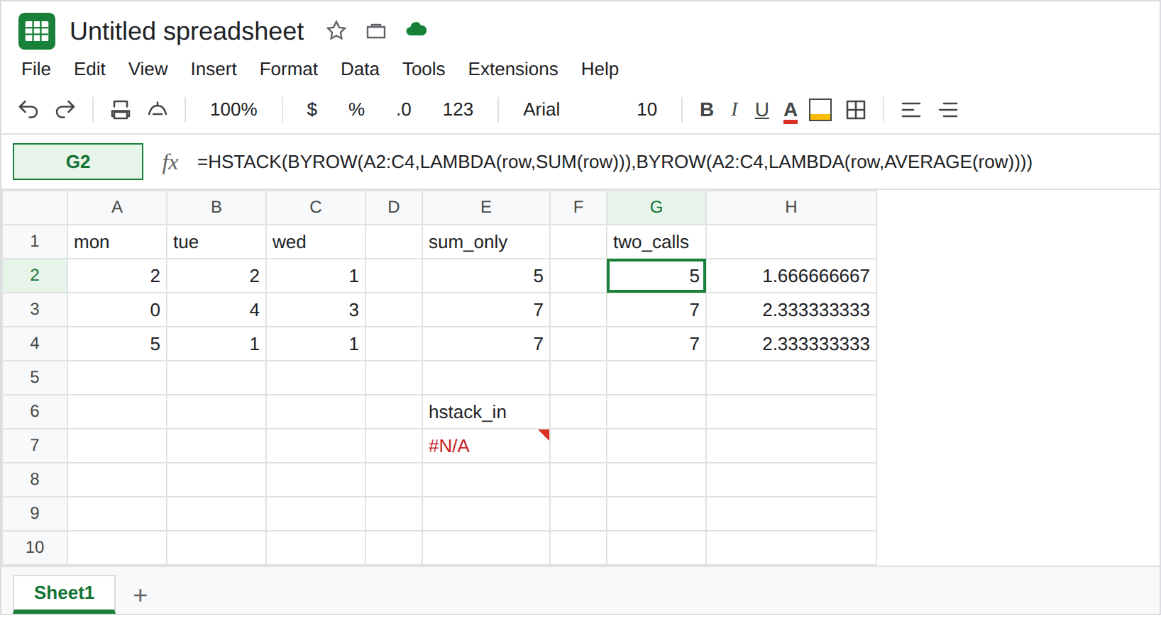
Two BYROW calls side by side. In G1 type two_calls. Leave G2:H4 empty. In G2 enter =HSTACK(BYROW(A2:C4,LAMBDA(row,SUM(row))),BYROW(A2:C4,LAMBDA(row,AVERAGE(row)))). G2:G4 is 5, 7, 7. H2:H4 is the three averages (1.666…). The HSTACK is outside. Each lambda returned one number. That block is the two-column control.

What is actually wrong

• BYROW collapses each row to a scalar, then spills those scalars down one column. A lambda that returns two numbers is a nested array. HSTACK, VSTACK, { }, and SPLIT all do that if they sit inside the lambda. E7 and E9.
• The same words outside the lambda are a different formula. G2 builds two one-column spills and places them next to each other. BYROW never saw a two-cell return.
• AVERAGE(row) alone would be a legal BYROW. The failure is the pair, not the average. A blank row’s SUM is 0. That zero is arithmetic, not this tooltip. See BYROW / MAP LAMBDA.
• MAP has the same nested-array rule. =MAP(A2:A4,LAMBDA(h,{h,h*2})) is the other page’s recreate. Do not switch E7 to MAP and return HSTACK.
• A blocked spill of a legal one-column BYROW is #REF! (Array result was not expanded). E7 never got that far. E7 failed inside the lambda. See array result was not expanded only if the tooltip names a cell.

Fix

Leave E7 and E9 broken. Leave E2 as 5 / 7 / 7.

One BYROW per metric, then HSTACK. Keep G2: =HSTACK(BYROW(A2:C4,LAMBDA(row,SUM(row))),BYROW(A2:C4,LAMBDA(row,AVERAGE(row)))). Sums in G, averages in H.

Or one grid from MAKEARRAY. =MAKEARRAY(3,2,LAMBDA(r,c,IF(c=1,SUM(INDEX(A2:C4,r)),AVERAGE(INDEX(A2:C4,r))))) returns the same two columns. Indexes start at 1. See MAKEARRAY LAMBDA if the lambda’s arity is the error instead.

Do not wrap E7 in IFERROR. You still have no average column. See IFERROR vs IFNA.

If the tooltip says Single value expected and the lambda contains HSTACK or { }, move that stack outside BYROW. If the lambda is SUM(row) and the tooltip names a cell below the formula, clear that cell.