A chart trendline shows no R² until Show R² is checked

A trendline is a chart setting on a series. It is off until you check it. Show R² is drawn only after the trendline exists, and only if that second box is checked. The equation and the R² are labels on the chart. They are not cells. A chart that already has a gray line and no R² is the first box without the second. A pie chart has no trendline block. Looking under Customize → Series and finding neither checkbox means this chart type does not offer one.

Error cells that gap the series are chart error gaps. The five-row LINEST block, including the cell that holds R², is LINEST verbose. Keep the Google Sheets UI in English. Sheet Error is an independent formula-error library, not a Google product.

Recreate it on a blank sheet

1. Open a blank spreadsheet. In A1 type x, B1 y. A2 1, B2 2. A3 2, B3 3. A4 3, B4 5. A5 4, B5 4. A6 5, B6 8. The points rise, with one step down at x 4, so a straight line will not sit on every point.

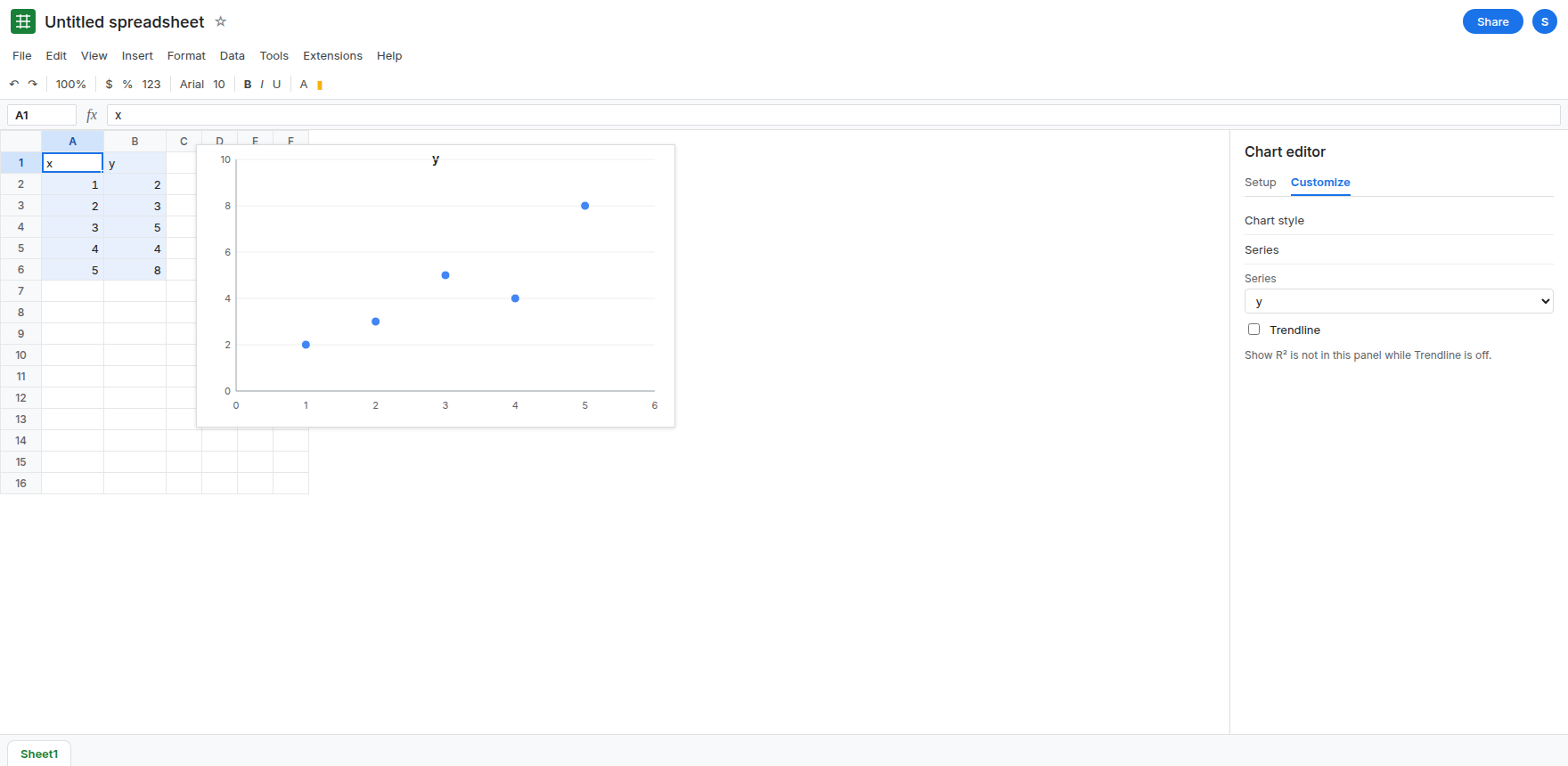
A scatter with no trendline. Select A1:B6. Insert → Chart. If the chart type is not a scatter, set Chart type to Scatter chart. You can use a line chart or a column chart for the same trendline control. Leave the chart with the five points and no extra line. Double-click the chart. Customize → Series. Scroll. Trendline is unchecked. There is no Show R² row yet. That absence is the recreate. Do not check the box until you have seen the panel without it.

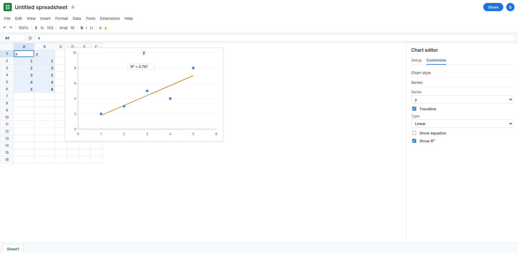
The line without the statistic. Check Trendline. A line appears through the points. Under the checkbox, Type appears (Linear is the default) and, with it, Show equation and Show R². Leave Show R² unchecked. The chart has a trendline and no R² label. That is the report people call “R² will not display.” The control is present. It is off.

Turn the label on. Check Show R². A label appears on the chart. It is a number between 0 and 1. This series is not a perfect line, so the label is not 1. You do not need to copy the digits into a cell. Uncheck Show R² again if you want the “missing label” picture to stay, after you have seen the label once. Check Show equation only if you also want the line’s equation as a second label. The equation is not R².

A pie has nowhere to check. Select A1:B6, Insert → Chart, Chart type Pie chart. Customize → Series has slice colors, not Trendline. A pie of these rows is the wrong chart. The missing checkbox is the chart type, not a hidden advanced menu. Delete the pie or set the type back to Scatter. See pie percent labels for what a pie does label.

What is actually wrong

• Show R² is created when Trendline is turned on. It is not a chart-wide switch in Customize → Chart style, and it is not on the Setup tab. A panel you opened before checking Trendline cannot show a box the editor has not added yet.
• The label is annotation. It does not land in a cell next to the chart. SUM of the chart is meaningless. If a formula needs R², use LINEST. With verbose TRUE, the statistics block includes that coefficient. Read the row before you quote it. See LINEST verbose.
• One series, one trendline. A combo with two series needs the series picker set to the series you mean. The other series can have Trendline off. See combo chart axis if the line looks flat for a scale reason. A flat line can still show an R² once the box is checked. The statistic does not fix the axis.
• #N/A in column B gaps or drops points. The trendline then fits a different set. That is chart error gaps. Show R² will label whatever fit remains. It does not explain a missing point.

This is not a spreadsheet locale. R² is not a TEXT format code.

Fix

Leave the scatter as the chart on A1:B6.

Check Trendline, then Show R². Double-click the chart. Customize → Series → select the y series if a dropdown lists more than one → check Trendline → check Show R². The label appears on the plot. Type can stay Linear. Change Type only when you meant a different fit. The R² changes with the type. It is still a label.

Put R² in a cell when the chart label is not enough. =INDEX(LINEST(B2:B6,A2:A6,TRUE,TRUE),3,1) returns the R² coefficient from the verbose block (third row, first column of that block). Confirm the cell against the chart label. If they disagree, the chart’s Type is not the linear fit LINEST just computed, or the ranges differ. See LINEST verbose.

Do not type an R² by hand onto the sheet and expect it to track new rows. The checkbox updates when the series updates. A typed number does not.

If Trendline is unchecked, Show R² is not missing. It is not on screen yet. If the chart type is a pie, switch to a scatter, line, or column. If you need the number in a cell, use LINEST.