

DATEVALUE of 03/04/2024 is a different day when the locale swaps month and day
Updated
DATEVALUE of a text date succeeds whenever both numbers can be a month. 03/04/2024 is legal on a United States spreadsheet and legal on a United Kingdom spreadsheet. The serials are not the same day. There is no red triangle. The sheet stored March 4 in one file and 3 April in the other, and both cells look formatted and finished.
This page is that silent swap. It is not DATEVALUE #VALUE!. That page is 13/1/2024 on a US locale, which cannot be a month, so the cell is #VALUE!. An error is easier to see than a date that is simply the other day. Keep the Google Sheets UI in English. Locale is File → Settings → Locale, not the display language, and not the country in your Google account.
Recreate it on a blank sheet
Section titled “Recreate it on a blank sheet”- Open a blank spreadsheet. File → Settings. Set Display language to English if it is not already. Set Locale to United States. Save. United States reads dates as month, then day, then year.
Text, not an auto-converted date. In A1 type text. In A2 type an apostrophe, then 03/04/2024, so the cell stays text. ISTEXT(A2) is TRUE. If you omit the apostrophe, Sheets may store a real date before DATEVALUE runs, and you will be formatting a serial you already built on the way in. The apostrophe is the recreate.
US parse. In B1 type us. In B2 enter =DATEVALUE(A2). Format B2 as a date if you only see a serial near 45355. The day is March 4, 2024. Month 3, day 4. No error. In B3 enter =TEXT(B2,"yyyy-mm-dd"). B3 shows 2024-03-04. That ISO string is the control for “which day did we actually get.”
The other ambiguous string. In A4 type an apostrophe, then 04/03/2024. In B4 enter =DATEVALUE(A4). On this US file B4 is April 3, 2024. =TEXT(B4,"yyyy-mm-dd") is 2024-04-03. Still no error. Two strings, two months, both accepted.
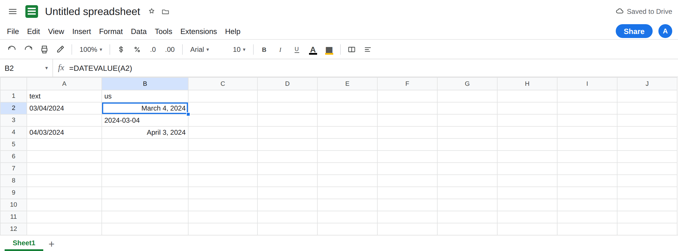
Switch the spreadsheet locale. File → Settings → Locale → United Kingdom. Leave Display language on English. B2 recalculates. The same text 03/04/2024 is now 3 April 2024. TEXT of B2 in yyyy-mm-dd is 2024-04-03. B4, which was April 3, is now 4 March 2024. Nobody edited the formulas. The file’s locale did.
The error case, so you do not mix the pages. In A6 type an apostrophe, then 13/04/2024. In B6 enter =DATEVALUE(A6). On United Kingdom, B6 is 13 April 2024. Set Locale back to United States. B6 becomes #VALUE!. The tooltip is DATEVALUE parameter ‘13/04/2024’ cannot be parsed to date/time. There is no month 13. That refusal is DATEVALUE #VALUE!. Put the locale back to whichever file you meant to document, and leave B2 as the ambiguous success. Do not “fix” B2 by hunting a triangle that is not there.
ISO text does not swap. In A8 type an apostrophe, then 2024-03-04. In B8 enter =DATEVALUE(A8). On both locales this is 4 March 2024. yyyy-mm-dd is not month/day versus day/month.
Leave B2 showing whichever day the current locale chose. Leave A2 as text.
What is actually wrong
Section titled “What is actually wrong”DATEVALUEdoes not have a month-first argument. It parses text with this spreadsheet’s locale. United States: the first number is the month. United Kingdom: the first number is the day. When both numbers are1through12, both readings are valid dates. The function is doing what the locale asked.- The viewer’s laptop does not decide. Locale is a file setting. A colleague who uses UK dates still gets the US reading when File → Settings → Locale is United States.
- Auto-conversion hides the text. Typing
03/04/2024without an apostrophe on a US sheet often becomes a date serial immediately.DATEVALUEof a serial is not the string bug.ISTEXTon A2 must stay TRUE or you are not recreating this page. 13/04/2024failing on a US sheet is a different lesson. The error proves the locale rejected a month. It does not prove that03/04/2024was read as 3 April. People see B6 break, conclude the locale is “working,” and trust B2. B2 never broke.- Read
TEXT(B2,"yyyy-mm-dd")when you need the day. A display format ofDD/MM/YYYYdoes not change the serial underneath.
This is not QUERY comparing dates. See QUERY date literal. This is not a comma versus semicolon Formula parse error. See locale parse error. B2 parsed. The serial is the bug.
This is not TO_DATE of a number. See TO_DATE serial. DATEVALUE here started from text.
Leave A2 and the US-or-UK B2 on the sheet so you can still see the swap. Set Locale to the convention this file is supposed to use, and do not keep flipping it to chase one cell.
Build the date from parts. In D2 enter =DATE(2024,3,4). D2 is 4 March 2024 on every locale. DATE takes year, month, day as numbers. It does not read a slash string. Use DATE when a formula, a form, or a CSV gave you the parts separately.
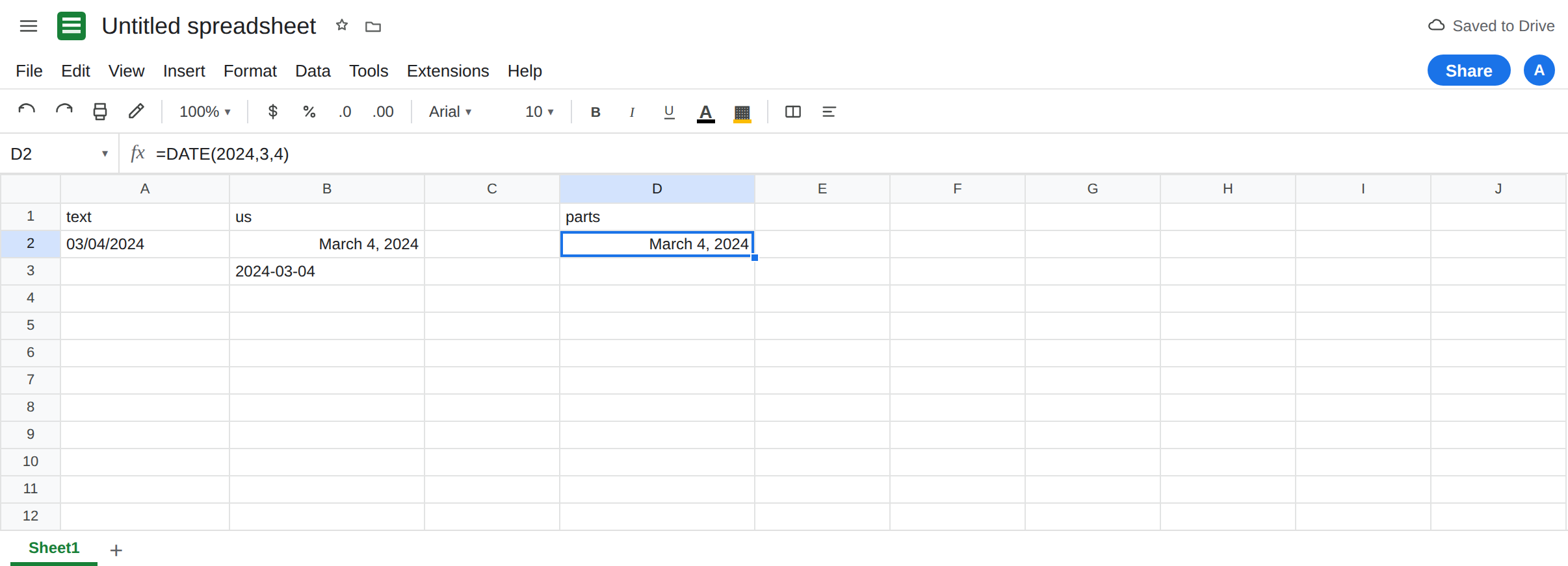
If the text is ISO, DATEVALUE is safe. B8 is the pattern: 2024-03-04. Prefer that shape in imports. If a partner must send slashes, make them send an unambiguous token (4 March 2024, or a column year, a column month, a column day) and call DATE.
Do not wrap B2 in IFERROR. There is no error to catch. IFERROR will not turn March into April. See IFERROR vs IFNA.
If DATEVALUE shows a date and the day of the month is the number you thought was the month, the string was ambiguous and the locale picked. Read yyyy-mm-dd. Replace the call with DATE or with ISO text. If the cell is #VALUE! because one number is greater than 12, you are on the other page.