

SUMPRODUCT of TRUE and FALSE stays 0 until you coerce them
Updated
SUMPRODUCT multiplies numbers and adds the products. A comparison such as A2:A5="East" produces TRUE and FALSE, not 1 and 0. Hand that array over with no arithmetic and the total can be 0. There is no triangle. The stores are on the sheet. Nothing was counted. Multiplying by 1, or the double unary --, turns TRUE into 1 and FALSE into 0. Then the same comparison counts.
Google Sheets sometimes coerces a boolean when it is already a separate numeric argument. Excel does not: the same formula is 0 there until you coerce. This page is the quiet zero, and the two forms that count in both products. A #VALUE! because the arrays have different shapes is SUMPRODUCT size. Keep the Google Sheets UI in English. Locale United States.
Recreate it on a blank sheet
Section titled “Recreate it on a blank sheet”- Open a blank spreadsheet. In A1 type
store, B1qty. A2East, B210. A3West, B34. A4East, B46. A5North, B51. Two East rows. Qty for East is16.
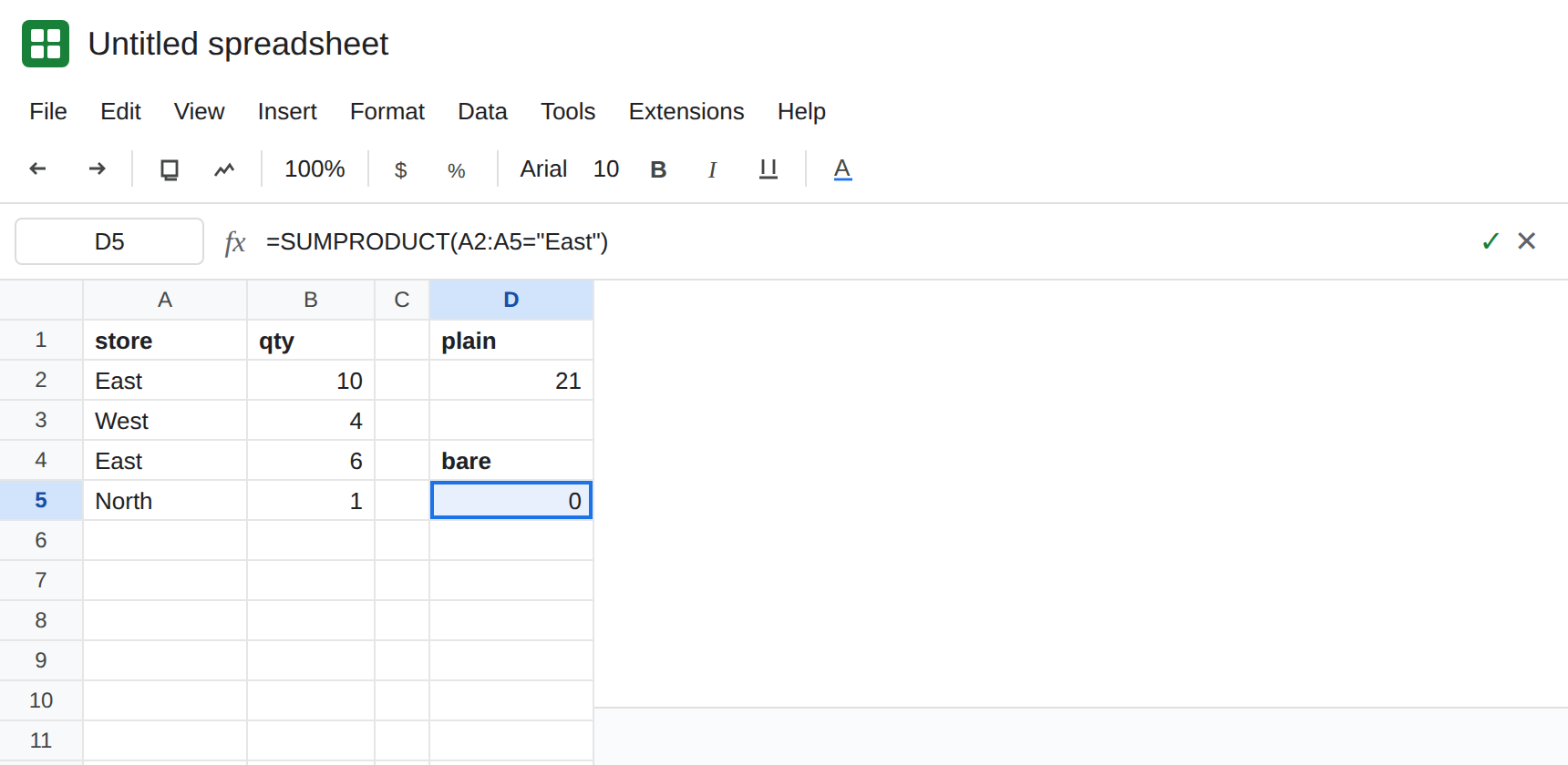
Numbers already coerce. In D1 type plain. In D2 enter =SUMPRODUCT(B2:B5). D2 is 21 (10+4+6+1). One numeric column. That cell is the control that SUMPRODUCT can add. It is not a conditional total.
A comparison with no arithmetic. In D4 type bare. In D5 enter =SUMPRODUCT(A2:A5="East"). Read D5. If it is 0, the booleans were not counted. Leave that 0. That is the broken total. If this Sheets account already shows 2, it coerced the array for you. Do not “fix” a 2. The Excel workbook with the same formula is still the 0 case, and the next cells are the forms that are 2 in both. Leave D5 as whichever number you got, and write down which one.
Multiply by 1. In F1 type times. In F2 enter =SUMPRODUCT((A2:A5="East")*1). F2 is 2. The parentheses build the comparisons first. *1 turns them into numbers. SUMPRODUCT adds those numbers.
Double unary. In F4 type unary. In F5 enter =SUMPRODUCT(--(A2:A5="East")). F5 is 2. The first - makes TRUE into -1 and FALSE into 0. The second - makes -1 into 1. Same count as F2.
A weighted total that never multiplies. In F7 enter =SUMPRODUCT((A2:A5="East"),B2:B5). In Excel this is 0 because the boolean argument is not numeric. In Google Sheets this shape often returns 16 already, because Sheets coerces that argument. If F7 is 0, you are in the Excel case (or a Sheets case that did not coerce). The form that is 16 in both is =SUMPRODUCT((A2:A5="East")*(B2:B5)). Put that in F9. F9 is 16. One array, products of 1 or 0 times qty. Leave F9 as 16.
Size is still #VALUE!. In H2 enter =SUMPRODUCT((A2:A5="East")*(B2:B4)). Four booleans times three qtys. #VALUE!. Tooltip: Array arguments to SUMPRODUCT are of different size. Coercion does not relax the shape. Leave H2 broken. See SUMPRODUCT size.
What is actually wrong
Section titled “What is actually wrong”TRUEis not the number1until a math operation says so. A bareSUMPRODUCTof the comparison has nothing to multiply. The documented Excel result is0. Sheets may already show the count. A zero with no triangle is this page. A2means this account coerced. It does not mean the Excel file will.*1and--are the same conversion.N(A2:A5="East")insideSUMPRODUCTis the same family. Use one of them and keep it. Do not stack--on a product that is already numeric.- Multiplying two comparisons,
(A2:A5="East")*(C2:C5="Open"), coerces because*is arithmetic. That product is1only on rows that pass both tests. A comma between them is not a multiply. The comma is howSUMPRODUCTlists arguments. F7 uses a comma. F9 uses*. - Text in a numeric slot becomes
0without a triangle when the shapes match. That quiet zero is one cell, not a failed condition. The size page showspcscounted as zero. Do not debug it as a boolean problem. #VALUE!with the different-size tooltip is the shape. H2. Adding--will not make three rows match four.
Leave D5 as the bare comparison so you can see whether it was 0. Leave H2 as #VALUE!.
Count with coercion. Keep F2 or F5. Both are 2. Prefer =SUMPRODUCT((A2:A5="East")*1) if you want the conversion to be obvious to the next reader. Prefer -- if that is the dialect the rest of the file uses. Do not use both in one formula.
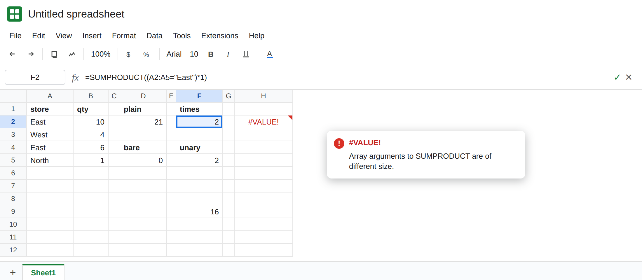
Sum a column with the condition. Keep F9: =SUMPRODUCT((A2:A5="East")*(B2:B5)) is 16. SUMIF(A2:A5,"East",B2:B5) is the same 16 without a coercion step. Use SUMIF when there is one condition. Use the product when you are already in SUMPRODUCT for several conditions.
In Excel, replace the bare comparison and the comma-separated boolean with the *1 or -- form before you trust a 0. Opening the same formula in Sheets and seeing 16 does not mean the Excel file was right.
Do not wrap D5 in IFERROR. The cell is not an error. It is a wrong total. See IFERROR hides cause.
If the total is 0 and the formula is a comparison with no *, coerce. If the tooltip says the arrays are different sizes, fix the ranges. If the total is already the count you wanted, this account coerced and the formula is not the bug.