SPARKLINE goes flat or disappears on blanks and #N/A

SPARKLINE scales the numbers it is given and draws one chart in one cell. Blank cells are not zeros. A blank in the middle leaves a gap or pulls the line in a way that looks flat next to a solid series. A #N/A in the same range is an error value. The sparkline often becomes #N/A and the chart disappears, or it drops that point in a way that no longer matches the series you think you plotted. Coercing the error to 0 draws a spike down to the axis that looks like a real zero.

An empty range, and an unknown charttype, are SPARKLINE empty / args. A bad color or type string is SPARKLINE charttype. Keep the Google Sheets UI in English. Sheet Error is an independent formula-error library, not a Google product.

Recreate it on a blank sheet

1. Open a blank spreadsheet. In A1 type clean. A2 3. A3 1. A4 4. A5 1. A6 5.

A line from numbers. In C1 type ok. In C2 enter =SPARKLINE(A2:A6). C2 shows a small line. That cell is the control.

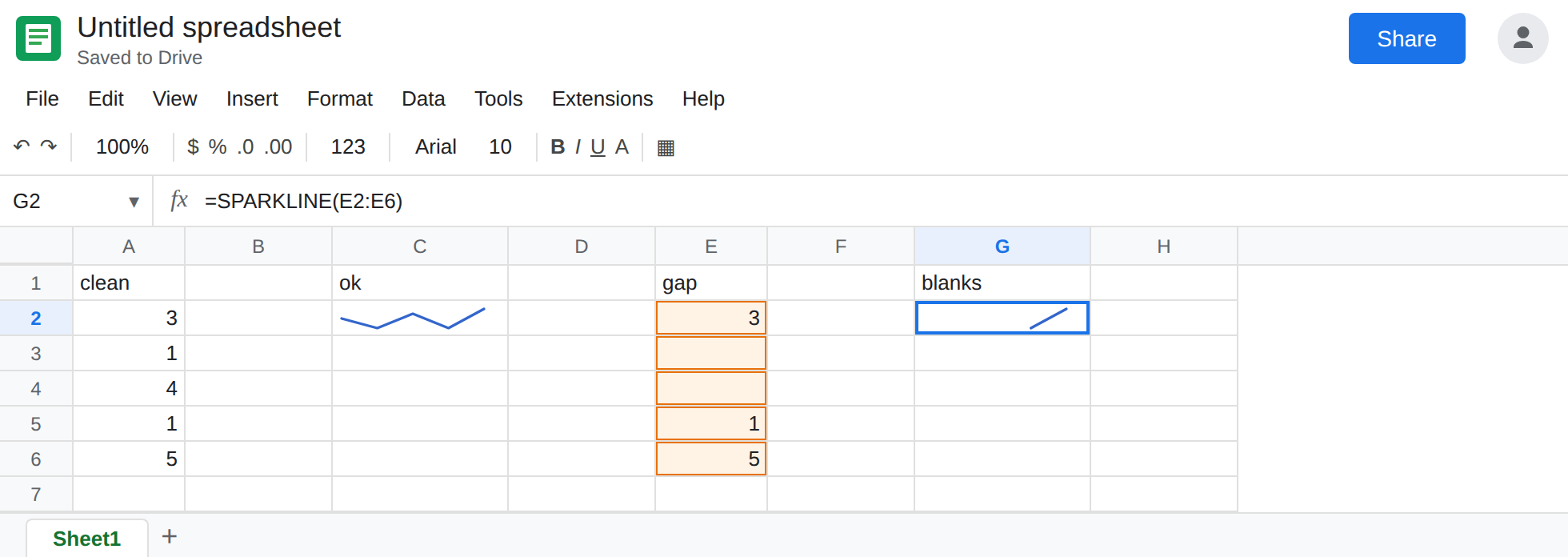
Blanks in the series. In E1 type gap. E2 3. Leave E3 and E4 blank. E5 1. E6 5. In G1 type blanks. In G2 enter =SPARKLINE(E2:E6). G2 still draws. The line is not the same shape as C2. Two missing points sit between 3 and 1. It can look almost flat if the remaining numbers are close, or like two stubs. It is not #N/A just for being partly empty. Leave G2 as that thinner chart.

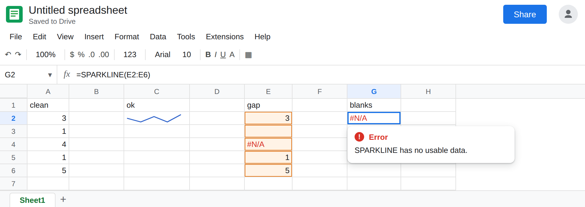
A #N/A in the series. In E4 enter =NA(). G2 now has 3, blank, #N/A, 1, 5 as its source. The sparkline cell goes to #N/A, or the line vanishes. The tooltip follows NA() (a #N/A you asked for) or says the sparkline has no usable data. Leave E4 as =NA() and leave G2 in that failed state.

Zero is a different picture. In I2 enter =SPARKLINE({3,0,0,1,5}). I2 draws a line that touches the bottom where the zeros are. That is a real zero in the data. It is what you get if you “fix” E4 with IFERROR(...,0) or IFNA(...,0). It is not a gap. Leave I2 as the contrast.

Empty is the other page. In K2 enter =SPARKLINE(A8:A10) with A8:A10 blank. #N/A because the range has no numbers. See SPARKLINE empty / args. Leave K2 broken.

Leave G2 failed. Leave C2 as the full line. Leave I2 as the zero dip.

What is actually wrong

• SPARKLINE does not treat blank as zero. G2 before the NA() still charts the numbers it has. The gaps are missing points, not measured zeros. I2 is what measured zeros look like.
• #N/A is not a blank. NA() is an error on purpose. See what #N/A means. Once that error is inside the data range, the sparkline has an error input. The chart is the wrong place to ignore it. G2 after E4 is that failure. A lookup #N/A in a cell of the range does the same thing.
• IFNA(E4,0) and IFERROR turn the error into a number the chart will plot. The line dives to zero. Readers think the metric crashed. The cell that was #N/A was “no measurement,” which is closer to a blank than to 0.
• A range that is all blanks is not this mixed case. K2 has nothing to scale. A bad "charttype" fails even on A2:A6. See SPARKLINE charttype.
• Options such as "nan" exist on some chart types to say how to treat non-numeric points ("convert" or "ignore" in the option map). A typo in that option is an invalid-option error, the charttype page, not a flatter line. Get the series clean before you tune options.

This is not IMAGE. A blank IMAGE cell is a URL. See IMAGE failed to load. G2 is a chart of cells.

Fix

Leave E4 as =NA() so the bad input stays visible. Leave K2 empty.

Plot numbers only. In G4 enter =SPARKLINE(FILTER(E2:E6,ISNUMBER(E2:E6))). ISNUMBER is false for blanks and for #N/A. The sparkline sees 3, 1, 5. It draws. It will not match C2 point for point, because the 4 and the gap were never numbers in column E. It will not be #N/A, and it will not dive to zero.

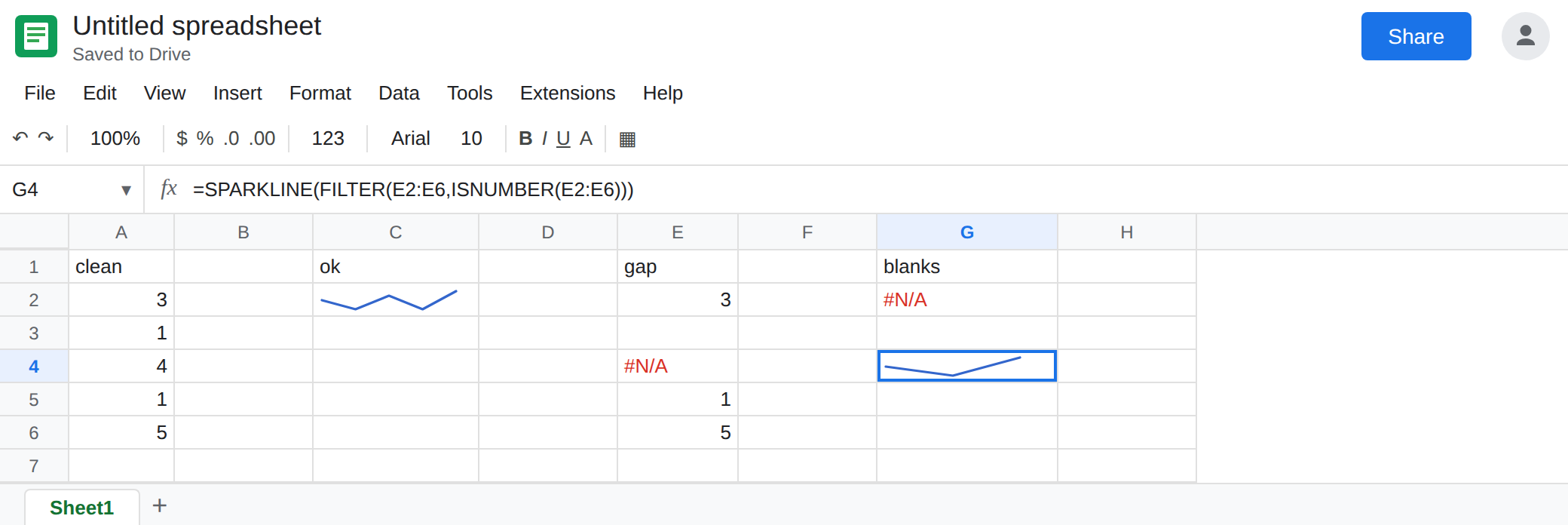
Gaps versus zeros. If a missing day should be a gap, keep it blank and out of the FILTER, as G4 does. If a missing day should be zero, put 0 in the cell on purpose and chart that column, the way I2 does. Do not use IFNA to invent the zero inside the sparkline unless a zero is the real measurement.

A whole blank range should stay blank or show a label, not a fake line: =IF(COUNT(E2:E6)=0,"",SPARKLINE(FILTER(E2:E6,ISNUMBER(E2:E6)))). COUNT ignores text and blanks. It also ignores #N/A only if you have already filtered, so prefer the FILTER inside once errors are possible.

Do not wrap G2 in IFERROR and a hardcoded sparkline of zeros. You would publish I2’s shape for a range that contains NA().

If the line sags where cells are blank, those blanks are not in the numeric series. If the cell is #N/A and one input is #N/A, filter to ISNUMBER or fix the lookup. If the range is completely empty, you are on the empty-range page. If the tooltip names charttype, you are on the charttype page.