Fix VLOOKUP #REF! in Google Sheets (column index bigger than the range)

VLOOKUP can return #REF! even when the lookup value is sitting on the sheet. This one is the column index: the third argument asks for a column the range does not have. It is not the #REF! you get after you delete a cell. The formula bar still shows VLOOKUP and a real range. The tooltip is an out of bounds range.

Recreate it on a blank sheet

1. Open a blank spreadsheet. In A1 type sku, B1 name, C1 price, D1 lookup, E1 result.
2. In A2 type 101. B2 Widget. C2 9.5. D2 101. In E2 enter =VLOOKUP(D2,A2:B2,3,FALSE). The cell shows #REF!.

E2 selected. Formula bar shows =VLOOKUP(D2,A2,3,FALSE). E2 is #REF! because index 3 is outside the two-column range A2.

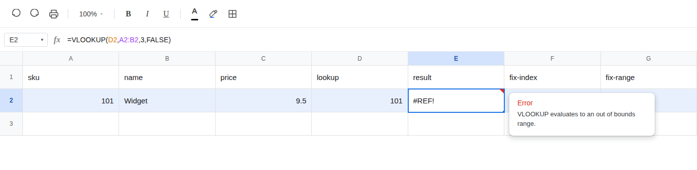
Leave E2 as the broken formula. Select it and read the formula bar. It is still =VLOOKUP(D2,A2:B2,3,FALSE). There is no #REF! inside the formula text.

Second recreate — index 4 on a three-column range. In E4 enter =VLOOKUP(D2,A2:C2,4,FALSE). A2:C2 is sku, name, price — three columns. Index 4 asks for a fourth. The cell shows #REF!. Same tooltip family. Widening the range from two columns to three did not help, because the index grew too. Leave E4 broken.

Price is on the sheet in C2. VLOOKUP will not walk into C on its own when the range stops at B, and it will not walk past C when the range stops at C.

What is actually wrong

A2:B2 is two columns wide. Index 3 asks for a third column that range does not contain. Column C is on the sheet, but it is outside the range you passed. The lookup itself can succeed. Sku 101 is in A2. The error is the return column, not a missing key and not a deleted reference.

Index 1 is the lookup column. Index 2 is the next column inside the range. The index is counted from the left of that range, not from column A of the spreadsheet. If you start the range at B (B2:C2), index 1 is sku and index 2 is price.

HLOOKUP does the same thing with a row index. =HLOOKUP(E3,B1:C2,3,FALSE) is #REF! because the range is two rows tall. See HLOOKUP #N/A / #REF!. Same error value. You are counting the other direction.

This is not a deleted reference. After a delete, #REF! appears inside the formula bar (=A1+#REF!). See after you delete. E2 still names D2 and A2:B2.

This is not a SORT or UNIQUE spill. A blocked array keeps a readable formula and the tooltip is Array result was not expanded. See SORT / UNIQUE spill. This is not a circular formula. See circular dependency. This is not IMPORTRANGE waiting for Allow access.

This is not #N/A. If the index were legal and the sku were missing, you would get #N/A. See what #N/A means. Do not wrap this #REF! in IFNA. IFNA will not catch it, and IFERROR will print “none” for a bad index as if the sku were absent. See IFERROR vs IFNA.

Fix

Leave E2 and E4 as the broken formulas so the error stays on the sheet. Put each fix in a neighboring cell.

• Want the name: change the index to 2. In F1 type fix-index. In F2 enter =VLOOKUP(D2,A2:B2,2,FALSE). The cell shows Widget.

• Want the price: keep index 3 and widen the range. In G1 type fix-range. In G2 enter =VLOOKUP(D2,A2:C2,3,FALSE). The cell shows 9.5.

F2 selected. Formula bar shows =VLOOKUP(D2,A2,2,FALSE) and F2 is Widget. E2 is still #REF!. G2 is 9.5 from =VLOOKUP(D2,A2,3,FALSE).

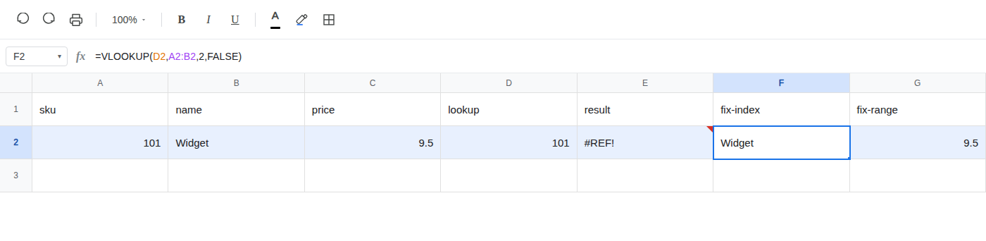
For E4, either drop the index to 3 (=VLOOKUP(D2,A2:C2,3,FALSE) — already in G2) or widen to four columns if a fourth column exists. Do not invent a column. Count the columns in the range before you pick the index. Index 1 is the lookup column. Index 3 needs a range at least three columns wide.