A CSV import leaves a leading apostrophe and VALUE or math returns #VALUE!

Some CSV fields arrive with a leading apostrophe as a real character: '1001, not the number 1001. The cell paints 1001 or '1001. The formula bar includes the quote. VALUE of that cell is #VALUE!. Adding 1 is #VALUE!. The id looks numeric. The first character is text, so the converters stop.

This page is that character. It is not CSV text vs number, where the apostrophe you type in Sheets is only a text prefix, LEN does not count it, and VALUE succeeds. Keep the Google Sheets UI in English. Sheet Error is an independent formula-error library, not a Google product.

Recreate it on a blank sheet

1. Open a blank spreadsheet. You can reproduce the leftover character without a file. In A1 type id. In A2 enter ="'1001". The formula stores five characters: apostrophe, then 1001. The formula bar on a selected result shows that quote if you look at A2 after the formula is evaluated — click A2 and read it. LEN is the check that does not depend on display. In B1 type len. In B2 enter =LEN(A2). B2 is 5, not 4.

VALUE and math fail. In C1 type value. In C2 enter =VALUE(A2). The cell shows #VALUE!. In D1 type plus. In D2 enter =A2+1. The cell shows #VALUE!. Tooltip on D2: expects number values. Leave C2 and D2 broken.

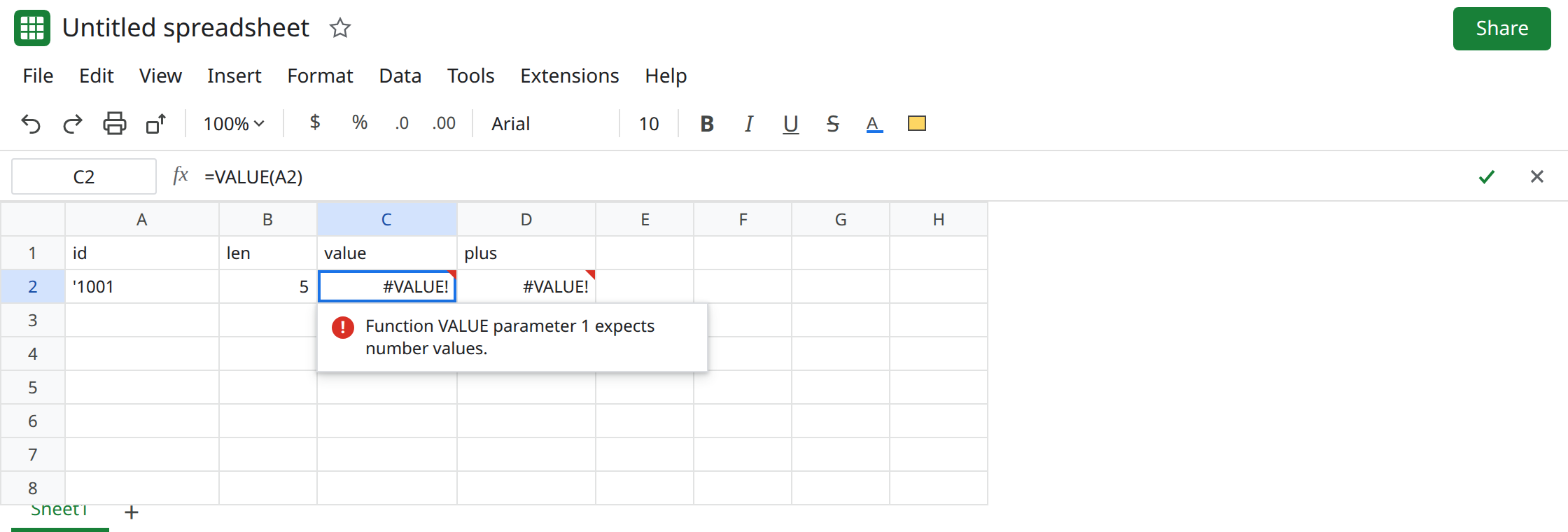
The import path that creates the same character. When you still have the file, File → Import → Upload. Choose the CSV. If a field in the file is the five characters '1001 (the quote is data, often written by an export that tried to force text), the imported cell matches A2: LEN is 5, and VALUE is #VALUE!. Unchecking Convert text to numbers, dates, and formulas keeps codes as text. It does not delete an apostrophe that is already in the field. Leave your imported cell broken the same way as C2.

Prefix only, so you do not mix the pages. In A4 type an apostrophe, then 1001, using the formula bar’s text prefix. Sheets consumes that prefix. In B4 enter =LEN(A4). B4 is 4. In C4 enter =VALUE(A4). C4 is 1001. Arithmetic on A4 often coerces. That row is not this bug. It is text versus a number, which breaks exact VLOOKUP. See CSV text vs number. Leave A2 as the five-character value.

SUM hides it differently. In D4 enter =SUM(A2). D4 is 0. SUM skips text. There is no triangle. The zero is not “no rows.” A2 is the id SUM refused. See SUMIF text numbers when the text is a plain number with no apostrophe. Here the first character is the quote.

What is actually wrong

• The import, or the ="'1001" recreate, put character code 39 in the value. VALUE parses numeric text. A leading apostrophe is not a thousands separator and not a sign. The parse fails, so C2 is #VALUE!.
• The prefix you type in the formula bar is an entry flag. It is not stored. LEN 4 versus LEN 5 is how you tell the pages apart. Cleaning a prefix that is not there will not fix a lookup miss.
• Convert text to numbers cannot repair a column whose cells already contain the quote. Conversion runs on the way in, and it still will not treat '1001 as 1001 when the quote is data.
• A trailing space fails VALUE too, and LEN is also one too high. CODE(LEFT(A2,1)) is 39 for an apostrophe. A space is 32. Strip the character you actually have.

This is not 10 + pcs as a generic type error, though the tooltip matches. See wrong type. A2 looks like an id. The extra character is the whole cause.

This is not VALUE("1.234,56") on a United States locale. See VALUE() locale. The apostrophe is not a decimal mark.

Fix

Leave C2 and D2 broken.

Strip the apostrophe, then convert. In F1 type clean. In F2 enter =VALUE(SUBSTITUTE(A2,"'","")). F2 is 1001. In F3 enter =F2+1. F3 is 1002. SUBSTITUTE removes every apostrophe in the cell. For a column, =ARRAYFORMULA(VALUE(SUBSTITUTE(A2:A2,"'",""))) on the real range, once LEN says the quote is present.

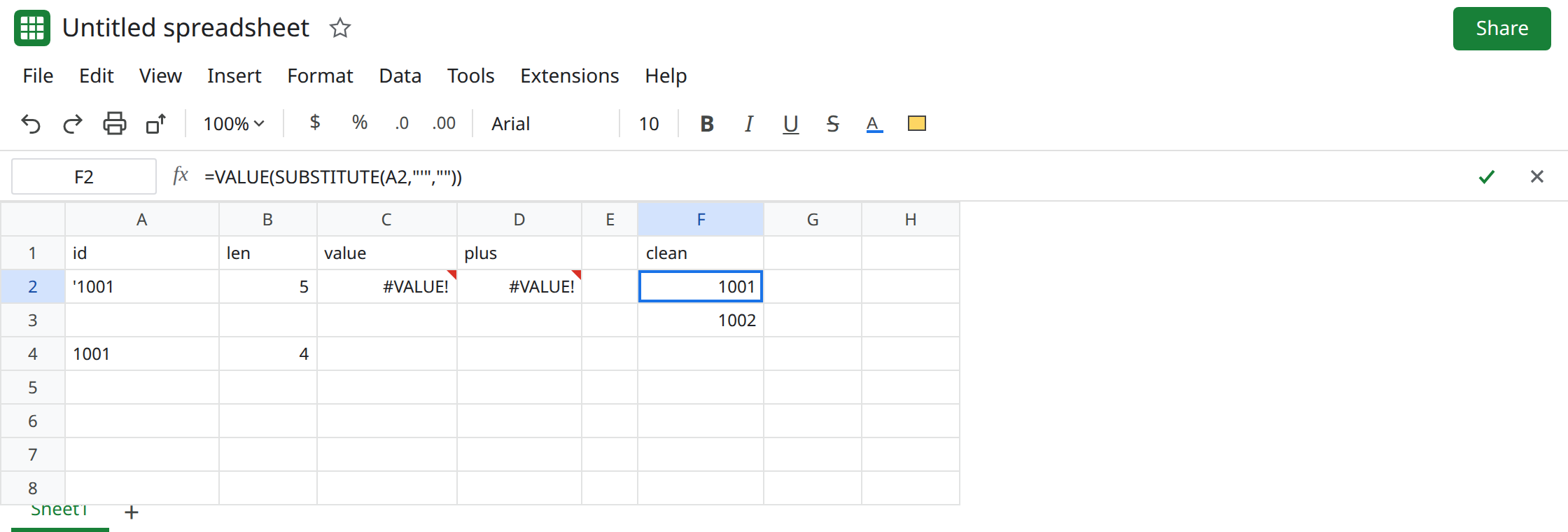
On the next import, remove the apostrophe in the export, or add the SUBSTITUTE helper and point math at the helper. Do not retype a leading apostrophe to “keep the id.” That prefix is the other page, and it is not what made VALUE fail here.

Do not wrap C2 in IFERROR. You would turn a dirty id into a blank and keep summing zeros. See IFERROR vs IFNA. IFNA does not catch #VALUE!.

If LEN is one more than the digits and CODE of the first character is 39, strip the apostrophe before VALUE. If LEN matches the digits and VALUE already returns the number, the lookup miss is text versus number, not this character.