

Power Query steps are dropped when an Excel file opens in Google Sheets
Updated
Power Query (Get & Transform) stores steps in the Excel workbook: the source, the filters, the rename, the load destination. Google Sheets does not run those steps. File → Import of the .xlsx keeps the values that were last loaded onto the sheet. The formula bar on those cells is empty. Changing the source file does not update the grid. There is no Queries & Connections pane and no Refresh that knows the M steps.
Sheet Error is not Microsoft and not Google. Keep the Google Sheets UI in English. A dynamic array that flattened to values is Excel spilled arrays become static. This page is a query that never arrived.
Recreate it on a blank sheet
Section titled “Recreate it on a blank sheet”- You need Excel for the first half. In Excel, put a tiny table on a sheet named
Source: A1sku, B1qty. A2101, B22. A3102, B35. Use Data → Get Data (or Data → From Table/Range) and load the result to a sheet namedLoadedwith Close & Load. In Excel, Data → Queries & Connections lists that query. Change B2 to9and refresh.Loadedshows9. That refresh is the control in Excel.
Save and open in Sheets. Save as .xlsx. In Google Sheets, File → Import → Upload and import the workbook. Open the tab that holds the loaded rows.
The values are here. The query is not. Click the cell that shows 101. The formula bar is empty. Click the cell that shows the quantity. Empty again. Data has no Queries & Connections list and no Refresh All for that import. Edit B2 on the Source tab if it came across. The loaded quantity does not change. Leave the loaded block as values.
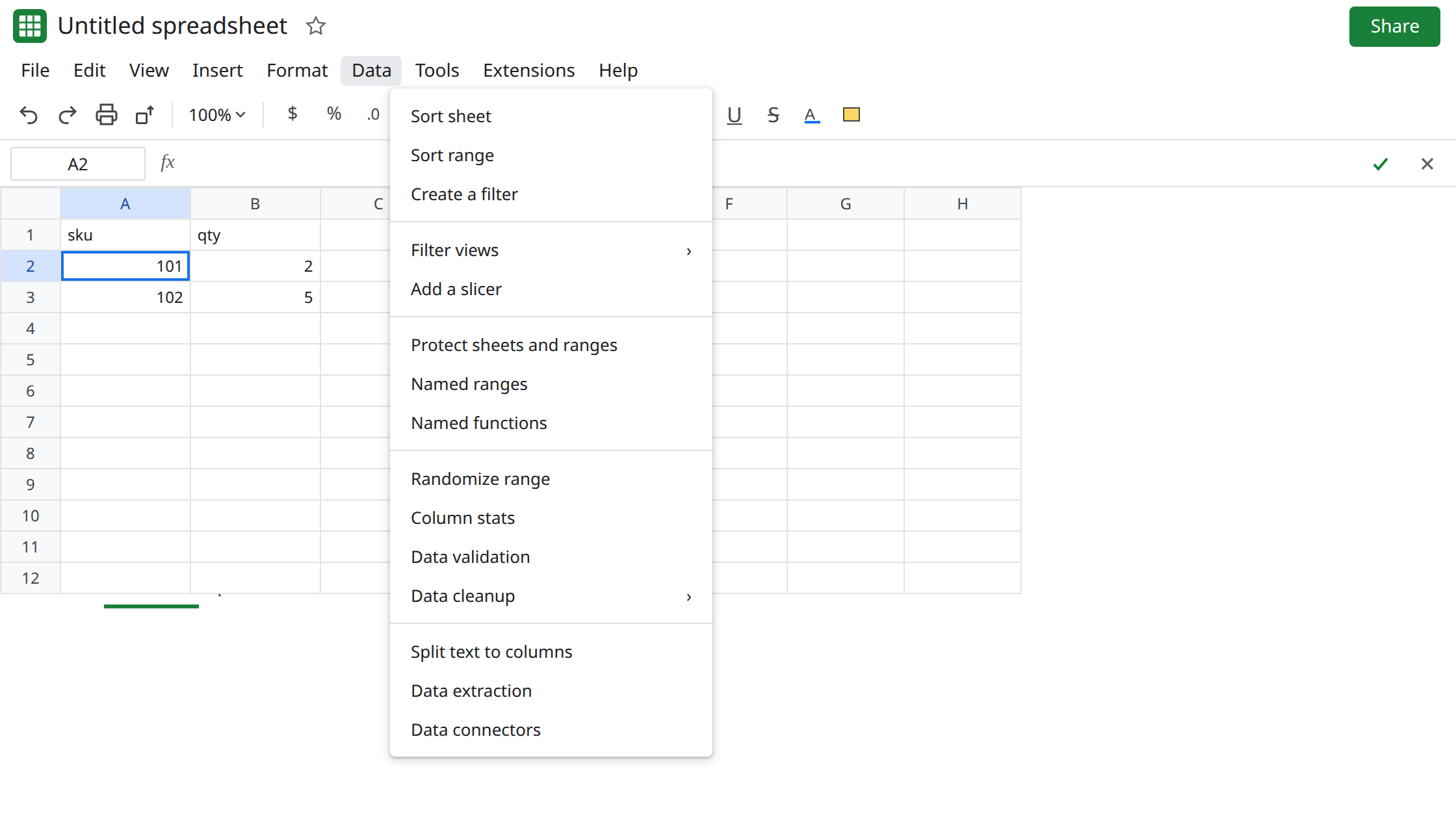
Sheets data connectors are a different product. Data → Data connectors (when your account shows it) connects Sheets to other Google data products. It does not open the Power Query steps inside this .xlsx, and it will not list the query name from Excel. Leave that menu. It is not a hidden Refresh.
A formula Sheets understands is a different import. If Loaded had been =SUM(Source!B2:B3) typed as a normal formula, the formula bar would still show SUM and edits would flow. Power Query output is not that formula. The empty bar is the test.
This is not IMPORTRANGE access. Nothing is asking you to Allow access. The steps were never a Sheets formula.
What is actually wrong
Section titled “What is actually wrong”- The query definition lives in the Excel package (the connection and the applied steps). Sheets’ importer reads worksheets. It writes the cached load as cells. Filters, merged columns, and renamed headers survive only as the values they produced at the last refresh in Excel.
- Refresh in Excel updates the
.xlsxon disk. The Sheets file is a copy from the moment of import. A later refresh in Excel does not push into the spreadsheet you already imported. Importing again replaces the grid with a new snapshot. It still does not install a live query. - People look for Data → Split text to columns or a pivot refresh. Those operate on cells that are already in Sheets. They cannot replay “remove this column, then change this type” from a query that is not on the file.
- If the loaded block was also an Excel table with
Sales[Qty]formulas, you have two losses. The steps are this page. The brackets are Excel table structured references.
This is not IMPORTDATA failing to fetch. That error is #N/A with a fetch tooltip, and the formula bar still shows IMPORTDATA. See IMPORTDATA fetch. An empty formula bar means there is no import formula to retry.
Leave the imported block as values so you can see that editing the source tab does nothing.
If the source is a CSV or TSV on a public https URL, load it with a Sheets import function. In a clear area, =IMPORTDATA("https://example.com/qty.csv") pulls the file when Sheets can fetch it. That formula refreshes on Sheets’ schedule. It does not replay M steps. Shape the result with QUERY or FILTER in the next cell. A URL that redirects or returns 403 is IMPORTDATA fetch, not a missing Power Query button.
If the source is another Google spreadsheet, use IMPORTRANGE and Allow access once. See IMPORTRANGE access. Then filter in Sheets.
If you only needed the snapshot, keep the values and stop looking for Refresh. Label the block so the next editor knows it will not track the workbook. Re-import when you want a newer snapshot, and expect the query to be dropped again.
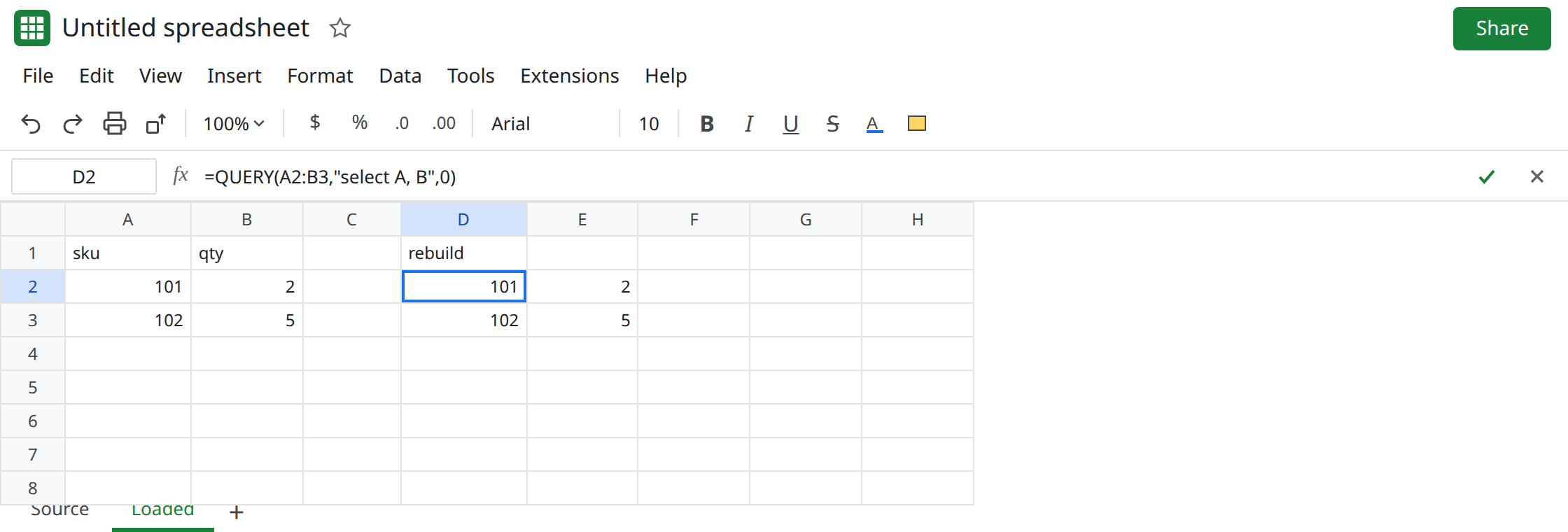
Do not wrap the value block in IFERROR. There is no error. The risk is a silent stale extract. See IFERROR hides cause.
If the formula bar is empty and Excel’s Queries pane was the thing that used to update those cells, the steps are gone. Rebuild the load with IMPORTDATA, IMPORTRANGE, or a formula on the values. If the bar shows IMPORTDATA and the cell is #N/A, you are on the fetch page.