QUERY + IMPORTRANGE NO_COLUMN in Google Sheets (use Col1, not A)

QUERY around IMPORTRANGE can still show #N/A when the import already works. select A is the usual column letter. On this array it is the wrong name. select B fails the same way. The import is not empty. The query language is naming columns the sheet-range way on data that is not a sheet range.

Connect the files first. If A1 is #REF! with You need to connect these sheets, that is IMPORTRANGE access. Click Allow access and wait for a spill before you debug QUERY.

Recreate it on a blank sheet

1. Source sheet: A1 sku, B1 name, A2 101, B2 Widget. Leave the tab named Sheet1. On the target spreadsheet, assume IMPORTRANGE from that source already works. Paste your source id where the formulas say SOURCE_ID.
2. In the target, A1 enter =QUERY(IMPORTRANGE("SOURCE_ID","Sheet1!A1:B2"),"select A",1). The cell shows #N/A.

A1 selected. Formula bar shows =QUERY(IMPORTRANGE("SOURCE_ID","Sheet1!A1"),"select A",1). A1 is #N/A. C1 is sku and C2 is 101.

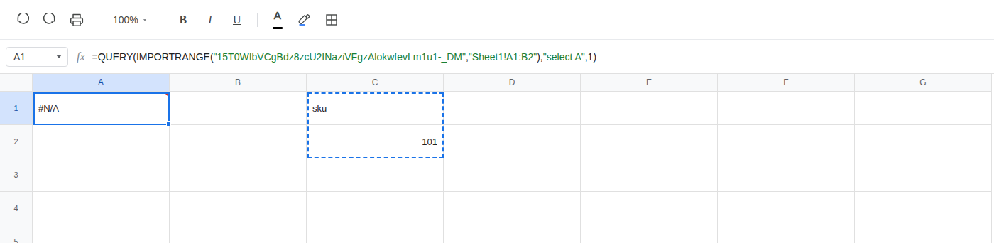
Leave A1 as the broken formula.

Second recreate — select B. In A4 enter =QUERY(IMPORTRANGE("SOURCE_ID","Sheet1!A1:B2"),"select B",1). The cell shows #N/A as well. B is not a missing name column. IMPORTRANGE has no column B. It has Col1 (sku) and Col2 (name). Leave A4 broken.

Check: =ERROR.TYPE(A1) is 7. That code is #N/A. The screenshot shows #N/A in A1; it does not show hover text. Some locales and older reports mention parse / NO_COLUMN wording for the same mistake. On an IMPORTRANGE wrapper the cell you actually get is commonly this #N/A, not the #VALUE! parse cell you get from QUERY({A1:B2},"select A",1) on a local array. That local-array parse is QUERY parse string.

What is actually wrong

QUERY is reading an IMPORTRANGE array, not a sheet range. Arrays do not have column letters A and B. QUERY numbers those columns Col1, Col2, … from the left of the imported array. The first imported column is Col1 even if it was column A on the source tab. The second is Col2 even if it was B.

select A is the syntax you use on a tab: =QUERY(Sheet1!A1:B2,"select A",1). Here it does not name a column, so the cell is #N/A. That is column syntax, not a missing lookup key. Sku 101 is on the source. VLOOKUP is not involved.

Wrapping extra braces does not switch you back to letters. QUERY({IMPORTRANGE(...)},"select A",1) is still an array. Still Col1. A sheet range that you wrap in { } (or FILTER, or another QUERY) also becomes Col1. Only a bare sheet range uses A.

This is not a lookup miss. See what #N/A means. There is no search value. This is not FILTER with zero rows. See FILTER no match. This is not mixed dates in a year() column. See QUERY mixed dates. This is not You need to connect these sheets. If the inner IMPORTRANGE alone already spills, permission is done.

This is not Result too large. See IMPORTRANGE too large. Get a small range working, then wrap QUERY.

Fix

Change select A to select Col1. QUERY numbers IMPORTRANGE columns Col1, Col2, … from the left of the imported array.

Leave A1 as the broken formula. In C1 enter =QUERY(IMPORTRANGE("SOURCE_ID","Sheet1!A1:B2"),"select Col1",1). The formula spills sku into C1 and 101 into C2.

C1 selected. Formula bar shows =QUERY(IMPORTRANGE("SOURCE_ID","Sheet1!A1"),"select Col1",1). C1 is sku and C2 is 101. A1 is still #N/A.

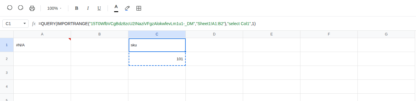
Leave A4 broken. In C4 enter =QUERY(IMPORTRANGE("SOURCE_ID","Sheet1!A1:B2"),"select Col2",1). The spill is name then Widget. select B becomes select Col2. Leave the rest of the QUERY as it is: the same where clauses, the same header argument 1.

Do not change File > Settings locale to fix this. Do not wrap A1 in IFNA until the column name is Col1. IFNA would print “none” for a syntax miss and look like an empty import. See IFERROR vs IFNA.