COUNTUNIQUE counts one formula blank, so the category total is one high

COUNTUNIQUE counts distinct values. It ignores cells that are truly empty, so a short list of skus with a few unused rows underneath is not inflated by those rows. A formula that returns "" is different. The cell looks blank, ISBLANK is false, and the zero-length string is a value. Every such cell is the same value, so they add one to the unique count, not one per row. Three real skus plus a column of formula blanks is 4. An auditor who asked for “categories that actually appear” expected 3.

COUNTA counts every non-empty cell, including each "", and does not care about duplicates. That page is COUNTA counts "". Distinct values that also have to pass a criterion are COUNTUNIQUEIFS range size. Keep the Google Sheets UI in English. Sheet Error is an independent formula-error library, not a Google product.

Recreate it on a blank sheet

1. Open a blank spreadsheet. In A1 type sku. A2 101. A3 102. A4 101. A5 103. Leave A6 and A7 truly empty. Do not type a space. Three distinct skus, and 101 is repeated.

Empty cells do not add a category. In C1 type plain. In C2 enter =COUNTUNIQUE(A2:A7). C2 is 3. The two empty cells are not a fourth sku. =COUNTA(A2:A7) is 4, because COUNTA counts the four filled cells and still counts 101 twice. C2 is the control for a range whose blanks are really empty.

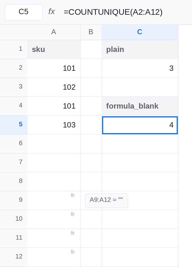
A formula blank is one extra unique. In A9 enter ="", and fill A9 down through A12. Four cells, each showing nothing. In C4 type formula_blank. In C5 enter =COUNTUNIQUE(A2:A12). C5 is 4. The skus are still 101, 102, and 103. The fourth unique is the zero-length string, counted once for all four formula blanks. =COUNTA(A9:A12) is 4, which is every formula blank, not the unique count. Leave C5 as 4.

One space is a different category. In A13 type a single space. In C7 enter =COUNTUNIQUE(A2:A13). C7 is 5. The space is not "" and it is not empty. It is its own unique. Leave C7 as 5 so the space stays visible as a separate problem from the formula blank.

The open column under an ARRAYFORMULA. In E2 enter =ARRAYFORMULA(IF(A2:A7="","",A2:A7)). E2:E5 repeat the skus. E6:E7 look blank because the IF returned "" for the empty source rows. In C9 enter =COUNTUNIQUE(E2:E7). C9 is 4, not 3. The spill did not add skus. It added the blank token. This is the dashboard pattern: a helper column “so the blanks stay blank,” then COUNTUNIQUE on that helper.

Leave C5 as 4. Leave C2 as 3.

What is actually wrong

• Truly empty cells are not values for COUNTUNIQUE. A2:A7 is 3. Extending the range over more empty rows does not keep adding one.
• ="" is a value. All of those cells share it, so the unique total rises by one, whether you have one formula blank or four. C5. ISBLANK(A9) is FALSE. The cell is not empty.
• A space is not that same value. C7 is 5. TRIM of a space is "", which then joins the formula-blank bucket instead of disappearing from the count. See the trim step below.
• COUNTA answers a different question. It counts cells that are not truly empty, duplicates included, formula blanks included. A unique count that matches COUNTA on a list with no duplicates and no formula blanks is a coincidence.
• Case is still distinct inside COUNTUNIQUE. 101 and a text variant are not this page. See UNIQUE case.

This is not COUNTUNIQUEIFS with a criteria range of the wrong height. That is #VALUE!. See COUNTUNIQUEIFS range size. C5 is a normal number. It is just one too high.

This is not UNIQUE spilling an extra blank row into a chart. =UNIQUE(A2:A12) will show the three skus and one blank row. COUNTUNIQUE is the count of that set. A blocked spill is SORT / UNIQUE spill.

Fix

Leave C5 as 4 so the extra unique stays on the sheet.

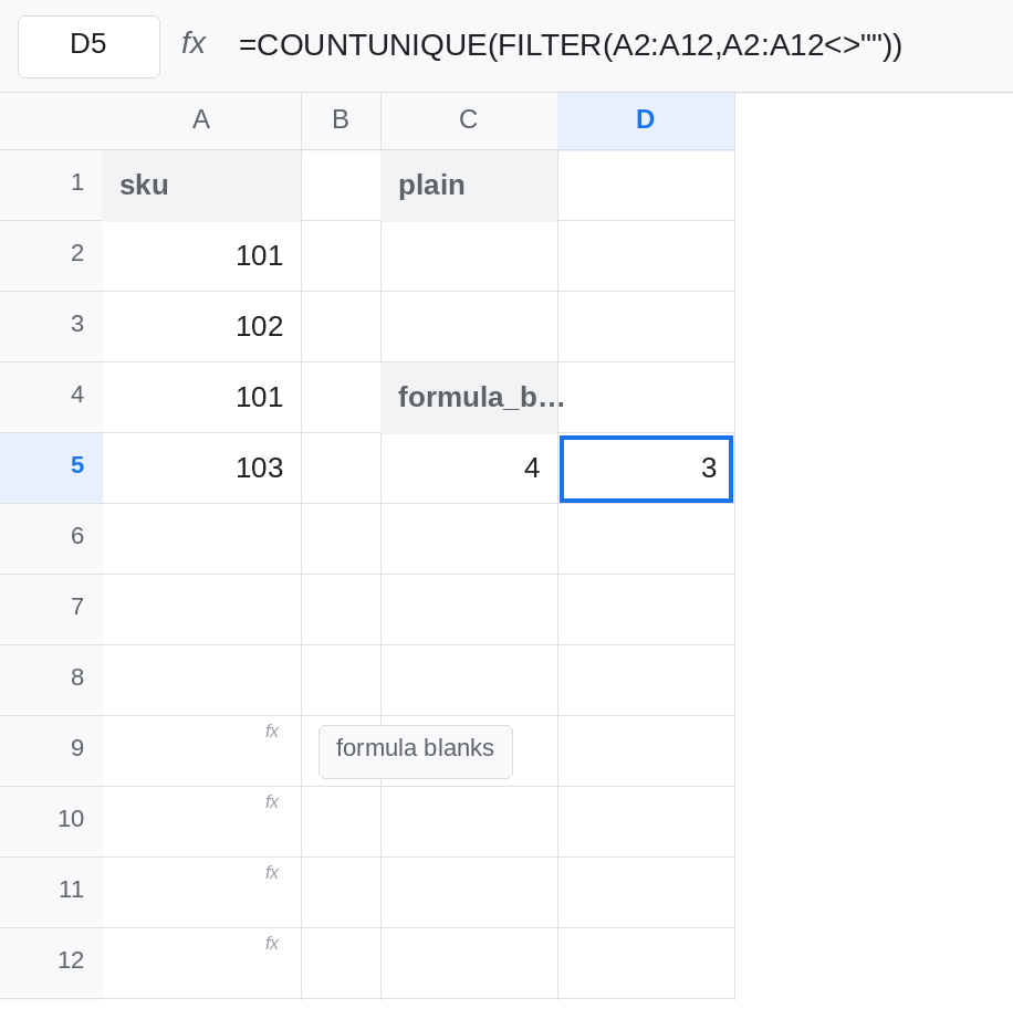
Drop zero-length text before the count. In D5 enter =COUNTUNIQUE(FILTER(A2:A12,A2:A12<>"")). D5 is 3. The filter removes "" and also removes truly empty cells. The space in A13 is not "", so include TRIM when spaces should not be categories: =COUNTUNIQUE(FILTER(A2:A13,LEN(TRIM(A2:A13))>0)). That cell is 3 as well. A non-breaking space survives TRIM. If the count stays high after TRIM, see CLEAN vs NBSP.

Same rule on the helper column. =COUNTUNIQUE(FILTER(E2:E7,E2:E7<>"")) is 3. Filtering the source skus is cleaner when you do not need the helper: =COUNTUNIQUE(A2:A5) was already 3 before the ARRAYFORMULA manufactured blanks.

No rows left. If every cell is "", FILTER returns #N/A and COUNTUNIQUE of that is #N/A. That means zero categories, which you may turn into 0 with IFNA around the FILTER only. See IFERROR vs IFNA and FILTER no match. Do not wrap the original COUNTUNIQUE in IFERROR. A real #VALUE! from a bad range would disappear into the same 0.

If the total is one higher than the skus you can see, check ISBLANK on a blank-looking cell. FALSE means a formula blank, and that blank is the extra unique. If ISBLANK is TRUE, the extra count is somewhere else: a space, a case variant, or a sku you scrolled past.