COUNTUNIQUEIFS returns #VALUE! when the criteria range is a different size

COUNTUNIQUEIFS(count_unique_range, criteria_range1, criterion1, …) counts distinct values in the first range, on rows that pass every criterion. The unique range and each criteria range must have the same number of rows and the same number of columns. A criteria range that is one row taller is #VALUE!. The tooltip is Array arguments to COUNTUNIQUEIFS are of different size. When the shapes match and nothing passes, the function returns 0. That 0 is “no rows,” not a size error.

COUNTIFS has the same size rule and does not count uniques. That page is COUNTIFS range size. UNIQUE of a filtered list is a different spill. Keep the Google Sheets UI in English. Sheet Error is an independent formula-error library, not a Google product.

Recreate it on a blank sheet

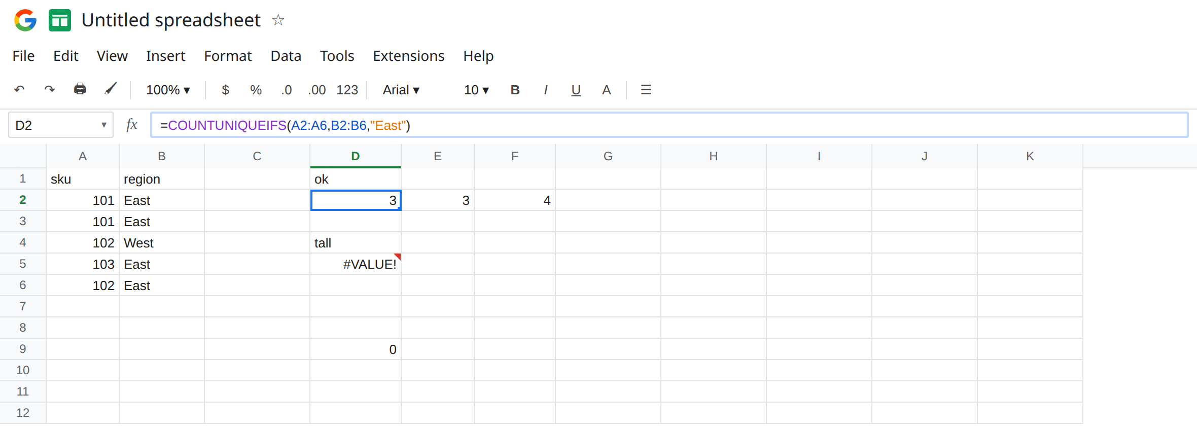
1. Open a blank spreadsheet. In A1 type sku, B1 region. A2 101, B2 East. A3 101, B3 East. A4 102, B4 West. A5 103, B5 East. A6 102, B6 East. Five data rows. East contains sku 101 twice, sku 103 once, and sku 102 once.

A count that works. In D1 type ok. In D2 enter =COUNTUNIQUEIFS(A2:A6,B2:B6,"East"). D2 is 3. The distinct East skus are 101, 103, and 102. The repeated 101 does not add a second unique. That cell is the control: same height, five and five.

Taller criteria range. In D4 type tall. In D5 enter =COUNTUNIQUEIFS(A2:A6,B2:B7,"East"). A2:A6 is five rows. B2:B7 is six. The cell shows #VALUE!. Tooltip: Array arguments to COUNTUNIQUEIFS are of different size. B7 is empty. Emptiness does not make the ranges the same shape. Leave D5 broken.

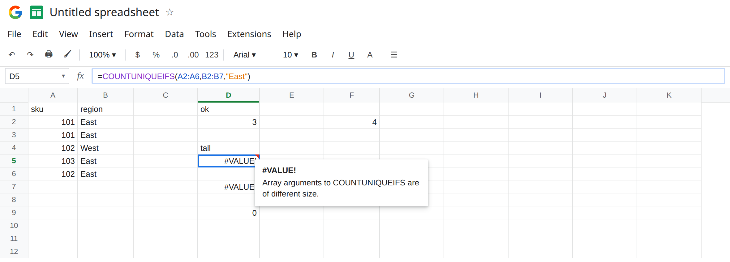
Open column against a closed one. In D7 enter =COUNTUNIQUEIFS(A2:A,B2:B6,"East"). A2:A runs to the bottom of the sheet. B2:B6 is five rows. #VALUE!, same tooltip. Leave D7 broken.

No match, same shape. In D9 enter =COUNTUNIQUEIFS(A2:A6,B2:B6,"North"). There is no North. The cell shows 0. There is no triangle. 0 means zero uniques survived the filter. It does not mean the ranges differ.

COUNTIFS is not this count. In F2 enter =COUNTIFS(B2:B6,"East"). F2 is 4 (four East rows, not three uniques). The extra East row is the duplicate 101. If your dashboard says 4 and the spec says “distinct skus,” you called COUNTIFS. Leave F2 as the contrast.

Shifted windows. In F5 enter =COUNTUNIQUEIFS(A2:A6,B3:B7,"East"). Both ranges are five rows. There is no #VALUE!. Sheets pairs A2 with B3, A3 with B4, and so on. The unique count is whatever those pairs produce, not the East uniques you can see in the table. Leave F5 as that quiet number. It is not D2’s 3 unless the shift happens to agree.

Leave D5 and D7 as #VALUE!. Leave D2 as 3. Leave D9 as 0.

What is actually wrong

• Every criteria range must match count_unique_range in both dimensions. Five next to six is #VALUE!. A single-column range next to a two-column range is the same error.
• An open end (A2:A or B:B) is thousands of rows. Pair it only with another open end that starts on the same row. A2:A with B2:B is legal. A2:A with B2:B6 is D7.
• Same height with a different start row does not error. F5 zips by position. A unique count that is “a bit off” with no triangle is often this shift, not a missing sku.
• No matching criterion is 0. North is 0 on purpose. Do not resize the ranges to chase a zero that is already a successful count of nothing.
• Duplicate keys inside the passing rows are the reason to use this function. COUNTIFS would say 4 East rows. COUNTUNIQUEIFS says 3 East skus. Both can be right. They are not interchangeable.

This is not FILTER mismatched heights, which is #N/A. See FILTER range size.

This is not COUNTUNIQUE of the whole sku column. =COUNTUNIQUE(A2:A6) is 3 as well on this tiny sheet (101, 102, 103) and it ignores region. The West row is included. If East and the whole column happen to share a number, check the criterion before you trust it.

This is not UNIQUE blocked by a filled cell. That spill is #REF!. See SORT / UNIQUE spill. D5 is #VALUE! before any spill.

Fix

Leave D5, D7, and F5 broken.

Use one rectangle. Keep D2: =COUNTUNIQUEIFS(A2:A6,B2:B6,"East"). In E2 enter =COUNTUNIQUEIFS(A2:A,B2:B,"East"). Both open, same start row. E2 is 3. Do not mix A2:A with B2:B6.

Two criteria stay the same shape. A status column in C2:C6 joins as =COUNTUNIQUEIFS(A2:A6,B2:B6,"East",C2:C6,"open"). Three ranges, one height. A status range of C2:C7 brings the tooltip back.

Read 0 as no rows. D9 does not need a new range. It needs a criterion that exists, or it needs to stay 0. Confirm with =COUNTIFS(B2:B6,"North"), which is also 0.

Do not wrap D5 in IFERROR and show 0. A size bug and a real empty region would look the same. See IFERROR vs IFNA. IFNA does not catch #VALUE!.

If the tooltip says different size, count the rows in each range in the formula bar, including open ends. If the cell is 0 and the shapes match, nothing passed. If the number is wrong and the shapes match, check whether one range starts a row lower (F5) and whether you wanted COUNTIFS row counts instead of distinct keys (F2).

Size vs zero vs COUNTIFS

D5 and D7 are #VALUE! (this page). D9 is 0 with matching ranges. F2 is 4 because COUNTIFS counts rows, not uniques. F5 is a same-size shift with no triangle. Fix the tooltip first. Then decide whether 0 or 3 or 4 is the number the header asked for.