Fix #NAME? in Google Sheets (unknown function or name)

#NAME? means Sheets does not recognize a name in the formula. Usually that name is a misspelled function. It can also be a named range or a named function that does not exist on this spreadsheet. The formula did not run.

Recreate it on a blank sheet

1. Open a blank spreadsheet. In A1 type sku, B1 name. A2 101, B2 Widget. D1 lookup, E1 typo, F1 ok. D2 101.
2. In E2 enter =VLOKUP(D2,A2:B2,2,FALSE) — one letter missing, VLOKUP not VLOOKUP. The cell shows #NAME?. The tooltip is Unknown function: ‘VLOKUP’.
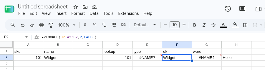
3. In F2 enter =VLOOKUP(D2,A2:B2,2,FALSE) with the correct spelling. The cell shows Widget.

Leave E2 as the broken formula so #NAME? stays on the sheet.

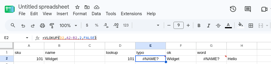
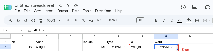
Second recreate — a bare word. In G1 type word. In G2 enter =Hello. The cell shows #NAME?. Sheets treats Hello as a function or named range. It is neither. In H2 enter ="Hello". The cell shows Hello. Quotes make a string. No quotes make a name.

What is actually wrong

• VLOKUP is not a function. VLOOKUP is. One missing letter is enough. Sheets does not fuzzy-match function names.
• The same error appears for any unknown name: =SUMM(A2), =XLOKUP(D2,A2,B2), a custom name you have not defined.
• Named functions (Data → Named functions) and named ranges (Data → Named ranges) are spreadsheet-local. Paste =TAX(A2) from another file and this file does not have TAX unless you create it here or import the named function. That is #NAME?, not #N/A.
• Function names in Google Sheets are English (VLOOKUP, SUM, IF) even when the UI is not. This is not Excel, where some locales use translated names. If the name is wrong, fixing the locale will not invent VLOKUP.

This is not a Formula parse error. A parse error is #ERROR! when the argument separators do not match the spreadsheet locale (commas vs semicolons). The function name can be spelled correctly and still fail to parse. See locale parse error. On this recreate the tooltip says Unknown function, and F2 with the same commas returns Widget.

This is not #N/A. #N/A means the function ran and found no match. See what #N/A means. E2 never got that far.

This is not #REF!. The ranges D2 and A2:B2 still exist. See after you delete.

Fix

Correct the name. In E2 the formula bar still shows VLOKUP. Change it to VLOOKUP, or keep E2 broken and use F2 as the working copy: =VLOOKUP(D2,A2:B2,2,FALSE) returns Widget.

For a bare word, either quote it (="Hello") or use a real function (=UPPER("Hello")). Do not leave an unquoted identifier unless it is a defined named range.

For a named function you brought from another spreadsheet: Data → Named functions, and define or import it on this file. For a named range: Data → Named ranges, and create the name, or replace it with a normal range like A2:B2.

Sheets function names are not case-sensitive. =vlookup(...) is fine. Spelling is not optional. IFNA is not IFNAA. ARRAYFORMULA is not ARRAYFORMUL.

Do not wrap #NAME? in IFERROR to hide it. The name is wrong. Fix the name.