SUMIFS wildcards match more rows than an exact criterion

SUMIFS criteria may contain * (any run of characters), ? (one character), and ~ (escape). The criterion "East" sums only East. "East*" sums East and Eastern. The criterion "N12*" sums every sku that starts with N12, including a sku whose name is exactly N12* and a sku named N12X. To sum the literal star, the criterion is "N12~*". The cell shows a total either way. There is no #N/A and no #VALUE! when the ranges match. The total is just larger than the one row you meant.

COUNTIF has the same wildcard rules. That page is COUNTIF literal * ?. VLOOKUP wildcards are VLOOKUP wildcards. A date stored as text is a different quiet zero: SUMIFS date text. Keep the Google Sheets UI in English. Sheet Error is an independent formula-error library, not a Google product.

Recreate it on a blank sheet

1. Open a blank spreadsheet. In A1 type sku, B1 region, C1 qty. A2 N12, B2 East, C2 10. A3 N12*, B3 Eastern, C3 20. A4 N12X, B4 West, C4 5. Three rows. The star in A3 is a character in the sku, not a pattern you typed in a formula yet.

Exact region. In E1 type exact. In E2 enter =SUMIFS(C2:C4,B2:B4,"East"). E2 is 10. Only B2. Eastern did not count. That cell is the control.

A star you added because you wanted “starts with.” In E4 type star. In E5 enter =SUMIFS(C2:C4,B2:B4,"East*"). E5 is 30. East 10 plus Eastern 20. The * means “then anything,” including “then nothing,” so East itself is included, and so is Eastern. If the header said “East only,” E5 is the wrong total and it will not turn red.

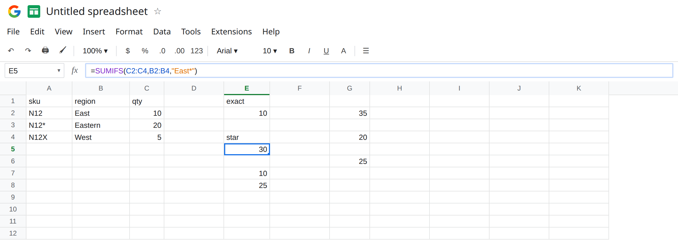
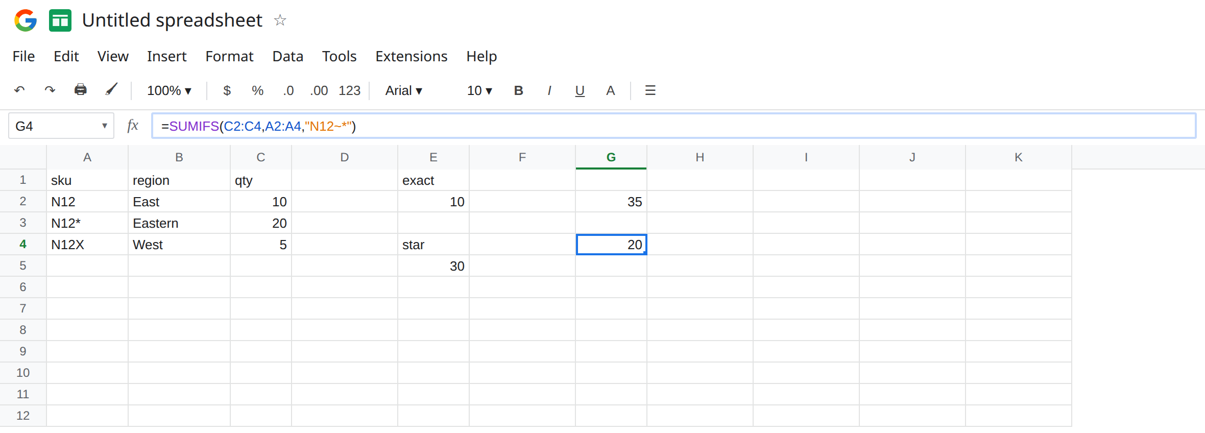
Sku pattern versus the literal star. In G2 enter =SUMIFS(C2:C4,A2:A4,"N12*"). G2 is 35. N12 (10), N12* (20), and N12X (5) all match, because * is a wildcard, not a search for the character *. In G4 enter =SUMIFS(C2:C4,A2:A4,"N12~*"). The tilde escapes the star. G4 is 20, only A3. Leave G2 as 35 so the unescaped pattern stays visible.

Question mark. In G6 enter =SUMIFS(C2:C4,A2:A4,"N12?"). ? is one character. N12X matches. N12 does not (no extra character). N12* matches, because the star is one character. G6 is 25 (20 + 5). A pattern that “looks like N12 plus the star key” is not one pattern.

Exact equals you do not need to spell with =. In E7 enter =SUMIFS(C2:C4,B2:B4,"=East"). E7 is 10, the same as E2. The leading = is optional for an exact text match. It does not turn wildcards off. "=East*" still has a star. In E8 enter =SUMIFS(C2:C4,B2:B4,"<>East"). E8 is 25 (Eastern and West). <> is “not equal,” and it is still an exact comparison, not a wildcard, unless you also type * .

Leave E5 as 30 and G2 as 35. Leave E2 as 10 and G4 as 20.

What is actually wrong

• In a SUMIFS criterion, * and ? are never literal unless a ~ sits in front of them. The same characters in the data are ordinary text. A3’s star does not “activate” anything until the criterion also contains a star.
• "East" and "East*" are different tests. The second includes the first. Adding a star to be safe always widens the sum. It does not make the match “more exact.”
• "N12~*" is the literal sku N12*. "N12~~" would be a literal tilde. A criterion that already ends in ~ because you were escaping something else needs a second tilde if you meant the character ~.
• Ranges that differ in height are #VALUE! before wildcards matter. See COUNTIFS range size. This page’s formulas all use three rows against three rows.
• A quiet 0 with an exact criterion usually means the text does not match: trailing space, East versus east is actually fine (SUMIFS text compares are not case-sensitive), or the date is text. Case will not split East and EAST. A space will. Wildcards do not trim. "East*" still fails on " East".

This is not QUERY contains. See QUERY contains / matches. contains is a different language. "East*" inside SUMIFS is not the matches regex.

This is not a SUMIF text-number miss. See SUMIF text numbers. The quantities here are numbers. The surprise is the pattern.

Fix

Leave E5 and G2 broken as the wide totals.

Use the pattern you mean, and escape stars that are data. Keep E2 for the region: =SUMIFS(C2:C4,B2:B4,"East"). Keep G4 for the starred sku: =SUMIFS(C2:C4,A2:A4,"N12~*"). If you truly want every sku that starts with N12, G2 is the right formula and the total 35 is honest — label the header sku prefix, not sku N12*.

Build the escape when the star comes from a cell. If H1 holds N12*, the criterion is "="&SUBSTITUTE(H1,"*","~*"). That turns the star into a literal before SUMIFS sees it. Substituting only when you mean a literal is the whole trick. Do not run that substitute on a prefix search.

Do not wrap E5 in IFERROR. The 30 is a successful sum of two regions. See IFERROR vs IFNA.

If the total jumped after you added *, you widened the criterion. If a sku that visibly contains * is missing from a prefix sum, you probably escaped it (~*) or you used ? and the tail is more than one character. If the total is 0 and the ranges match, the text does not match — check spaces before you add another star.

Exact, star, and tilde

E2 "East" is 10. E5 "East*" is 30. G2 "N12*" is 35 across all three skus. G4 "N12~*" is 20, only the sku that contains a star. E7 "=East" matches E2. The = does not disable wildcards. COUNTIF on the same criteria counts rows instead of summing quantities. See COUNTIF literal * ?.