Conditional formatting formulas lock the wrong row when both $ are absolute

A conditional formatting custom formula is not an ARRAYFORMULA. You write it as if it sat in the top-left cell of the apply-to range. Sheets then fills it down and across. $ locks a column, a row, or both, the same way it does in a normal fill. =$A$2="East" locks row 2. Every formatted row still asks whether A2 is East. The West row lights up because A2 is East, not because A3 is East.

Recreate it on a blank sheet

1. Open a blank spreadsheet. Keep the Google Sheets UI in English. In A1 type region, B1 hours. A2 East, B2 10. A3 West, B3 4. A4 East, B4 8.

Open the rule. Select A2:B4. Format → Conditional formatting. The apply-to range reads A2:B4. Format rules: Custom formula is. Do not pick “Text is exactly.”

Both locks. In the formula box enter =$A$2="East". Pick any fill color. Click Done. If A2 is East, the entire range A2:B4 is filled, including A3:B3 where the region is West. The rule never read A3 or A4. Change A2 to West. The whole fill disappears, including the East in A4. Put A2 back to East so the bad fill returns.

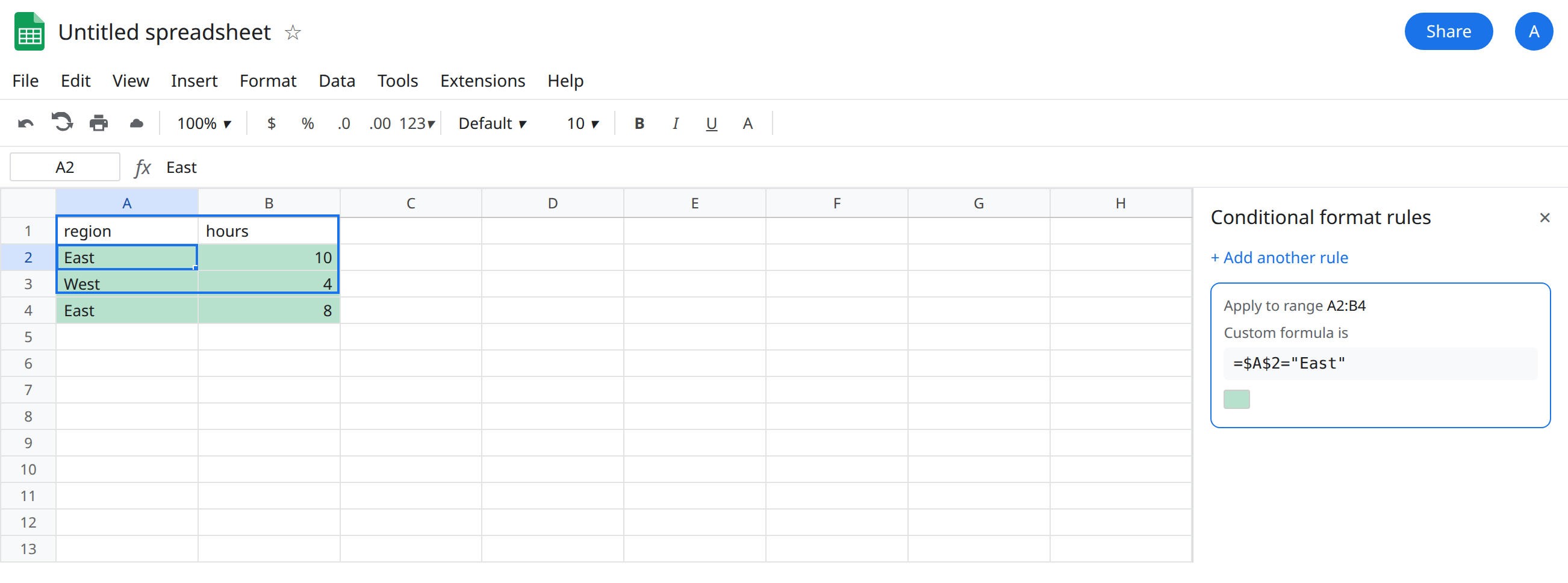
Column lock only. Edit the rule. Change the formula to =$A2="East". Done. A2:B2 and A4:B4 are filled. A3:B3 is not. Row 3 tests $A3, because the row was relative and the fill moved it. Column A stays locked, so the hours cell B2 tests $A2, not B2. Hours 10 is not the word East, and the row still fills. That is the lock doing the right job.

No lock on the column. Edit the formula to =A2="East" with no dollar signs. A2 and A4 still fill. B2 and B4 do not: when the formula is evaluated on B2 it has become =B2="East", and 10 is not East. The region column looks correct. The hours column looks like the rule is broken. The rule filled relatively, which is what you asked for.

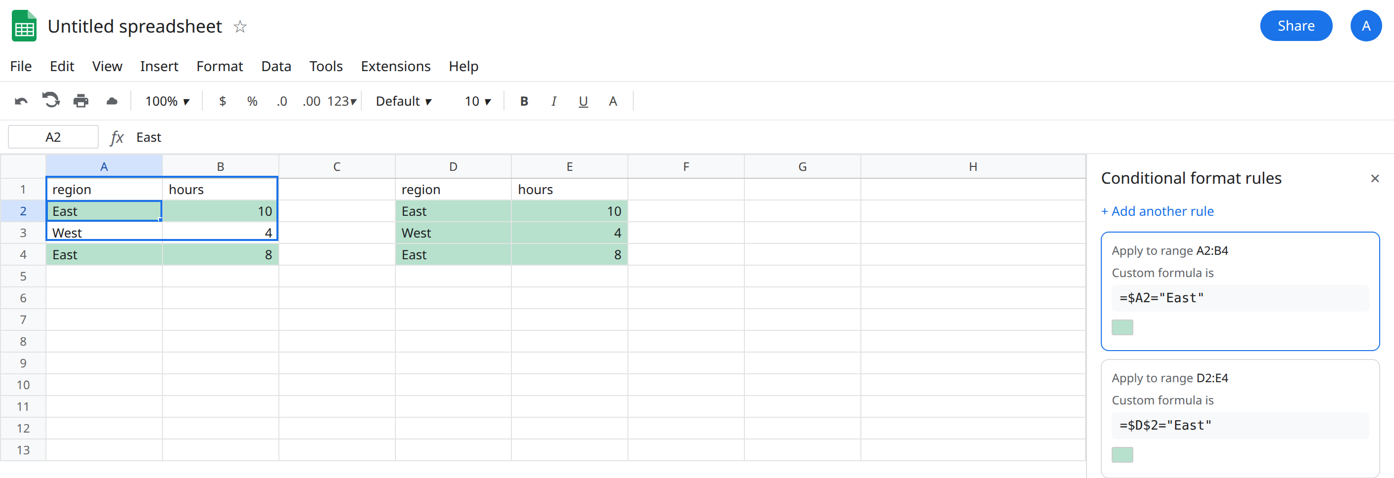
Leave the absolute rule in a second range so you can see both. Copy A2:B4 to D2:E4. Add a second rule on D2:E4 with =$D$2="East". That block fills every row. The first block, with =$A2="East", does not.

There is no error triangle. Conditional formatting does not return #N/A when the test is false. It returns no fill.

What is actually wrong

• The formula is stored once, for the top-left cell of the apply-to range. Here that cell is A2. =$A2 in A2 means “column A, this row.” Filled to A4 it means A4. =$A$2 filled to A4 still means A2. The West row is highlighted because it never had its own test.
• The apply-to range and the formula must start on the same row. If the range is A2:B4 and you write =$A1="East", row 2 of the sheet tests A1 (the header). The header is not East, so nothing fills, including the East data. People then add more dollar signs. The row number in the formula should be the first row of the range.
• Dollar signs are independent. $A2 locks the column. A$2 locks the row and lets the column move, which is the wrong pair for “highlight the row when column A says East.” $A$2 locks both. The recreate that paints West is the double lock.
• Two columns make the column lock visible. A rule applied only to A2:A4 can use =A2="East" with no $ and look fine, because fill-down stays in column A. The moment the range grows to include hours, the unlocked column drifts. Put $ on the column when the test must stay on region.
• Do not wrap the test in ARRAYFORMULA. The format engine already fills. ARRAYFORMULA in a custom formula is not the spill you get in a cell, and it is the wrong tool. A spilled FILTER of East rows is FILTER OR vs AND or a plain FILTER, not a paint rule.
• Text must match. East with a trailing space fails =$A2="East" and the row stays bare. That looks like a $ bug. =LEN(A2) is the check. See CHAR(160) blanks when the space is not a normal space.
• The rule does not use the case-sensitive EXACT unless you write EXACT. east and East match with =.

Fix

Keep one broken rule on D2:E4 (=$D$2="East") so the painted West row stays in the file.

Lock the column, not the row. On A2:B4 the formula is =$A2="East". First row of the range is row 2, so the formula says A2, not A1 and not $A$2.

Apply to the column you test, if you do not want to think about $. Range A2:A4 and formula =A2="East" stays in column A as it fills down. Add $A before you widen the range to column B.

A numeric test uses the same fill. =$B2>9 on A2:B4 fills rows whose hours are greater than 9 (the East 10 row only, in this sheet). $B$2 would paint every row whenever B2 is greater than 9.

Do not put IFERROR around the custom formula. A false test should be unpainted, not a swallowed error. If the formula itself is illegal, the rule does nothing and the pane does not show a cell tooltip. Fix the formula in a normal cell first: in G2 enter =$A2="East" and fill it down. G2 TRUE, G3 FALSE, G4 TRUE. Paste that formula into the rule.

If every row in the range paints together, a $ is locking the row. Delete the dollar sign in front of the row number and keep the one in front of the column when the test has to stay put.