

Fix FIND and SEARCH #VALUE! in Google Sheets (substring not found)
Updated
FIND and SEARCH return a number: the position where a substring starts. When that substring is not in the text, there is no position. Sheets returns #VALUE!, not #N/A. The formula ran. The needle is not in the haystack. FIND is case-sensitive. SEARCH is not.
This page is a substring miss. It is not REGEXEXTRACT #N/A (a regex that does not match, error value #N/A). It is not wrong type as a generic 10 + pcs primer, though the error value is the same family.
Recreate it on a blank sheet
Section titled “Recreate it on a blank sheet”- Open a blank spreadsheet. In A1 type
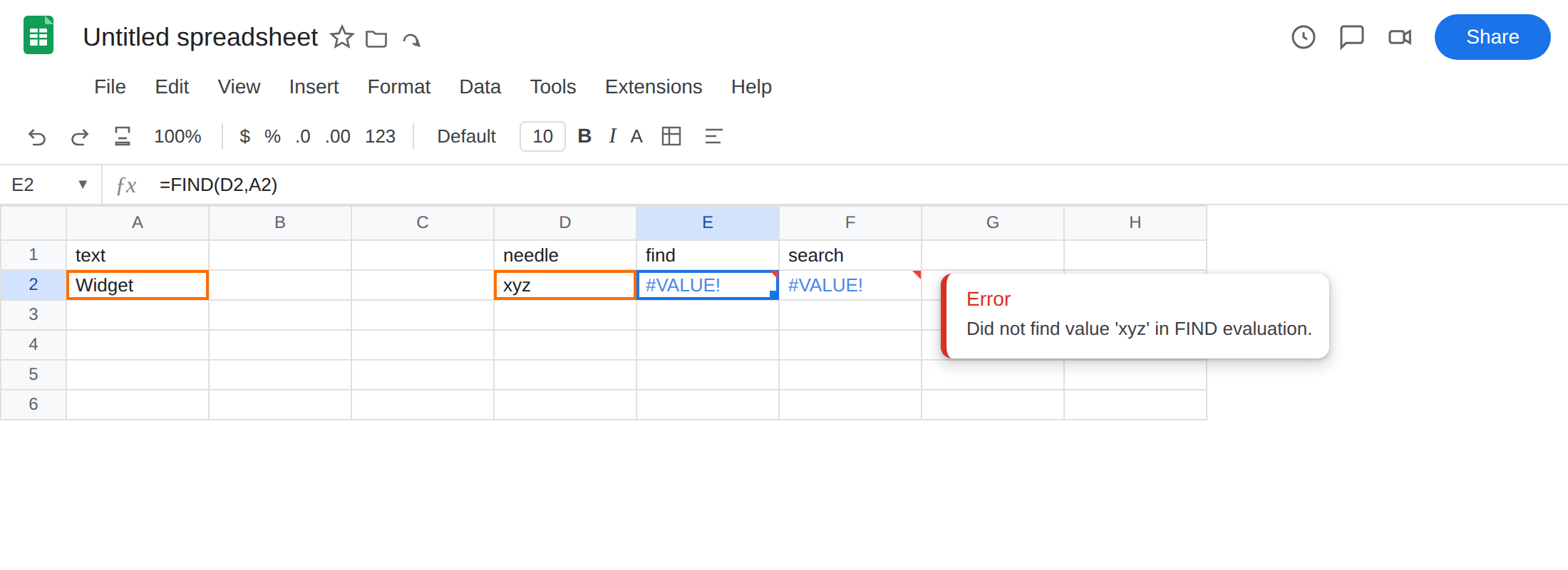
text. In A2 typeWidget. D1needle, E1find, F1search. - A miss both functions share. In D2 type
xyz. In E2 enter=FIND(D2,A2). The cell shows#VALUE!. In F2 enter=SEARCH(D2,A2). The cell shows#VALUE!.xyzis not in Widget. Leave E2 and F2 broken.
- Case:
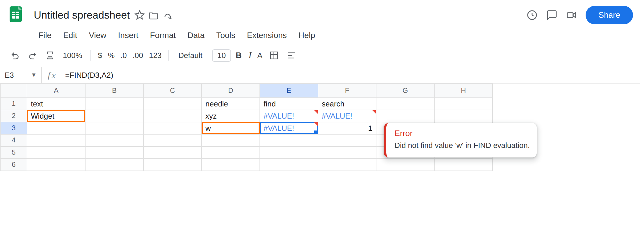
FINDmisses,SEARCHhits. In D3 typew(lowercase). In E3 enter=FIND(D3,A2). The cell shows#VALUE!.FINDwill not treatwasW. In F3 enter=SEARCH(D3,A2). The cell shows1.SEARCHignores case. Widget starts with W. Leave E3 broken. F3 is the control for “same letters, different function.”
- A case-sensitive hit. In D4 type
W. In E4 enter=FIND(D4,A2). The cell shows1. Same text as E3 except the needle’s case. That row provesFINDworks when the case matches.
SEARCH wildcards (not FIND). In D5 type W*t. In F5 enter =SEARCH(D5,A2). SEARCH treats ? and * as wildcards. This often returns 1. In E5 enter =FIND(D5,A2). FIND looks for a literal asterisk. E5 is #VALUE! unless Widget actually contains W*t. Leave E5 as that contrast if it errors.
Do not wrap yet. Read E2 versus F3: both can be #VALUE!, but F3 is not.
What is actually wrong
Section titled “What is actually wrong”FIND(needle, text)andSEARCH(needle, text)fail when the needle never occurs. The return type is a position. No occurrence means#VALUE!.FINDcompares case.wis notW.SEARCHdoes not. That is why E3 errors and F3 is1.- Empty needle is a different refusal (
FIND("",A2)is#VALUE!in Sheets). A blank D2 is not “found at position 1.” Type a real substring. - The optional start position (
FIND(needle, text, start)) does not create a match.=FIND("W",A2,2)starts after the first character and then misses — still#VALUE!, not a wrap-around. SEARCHwildcards can hide a miss you meant to be literal. If you needed a literal*or?,FINDis the function, or escape the wildcard inSEARCH(~*,~?).
This is not REGEXEXTRACT #N/A. REGEXEXTRACT("Widget","xyz") is #N/A. REGEXMATCH("Widget","xyz") is FALSE. Extract returns matched text, so a miss is the lookup-style error. FIND / SEARCH return a number, so a miss is #VALUE!. See REGEX no match. Do not debug E2 as a regex miss. Do not debug a REGEXEXTRACT #N/A with FIND.
This is not a lookup miss. VLOOKUP / XLOOKUP / MATCH / FILTER use #N/A. See what #N/A means, XLOOKUP #N/A, MATCH #N/A.
This is not DATEVALUE refusing a locale date string. See DATEVALUE locale. Widget is not a date.
Leave E2, F2, and E3 broken so #VALUE! stays on the sheet.
Confirm the text contains the needle. Change D2 to idg. E2 becomes 2. Put xyz back. If toggling the needle makes #VALUE! come and go, the functions work and the substring is absent.
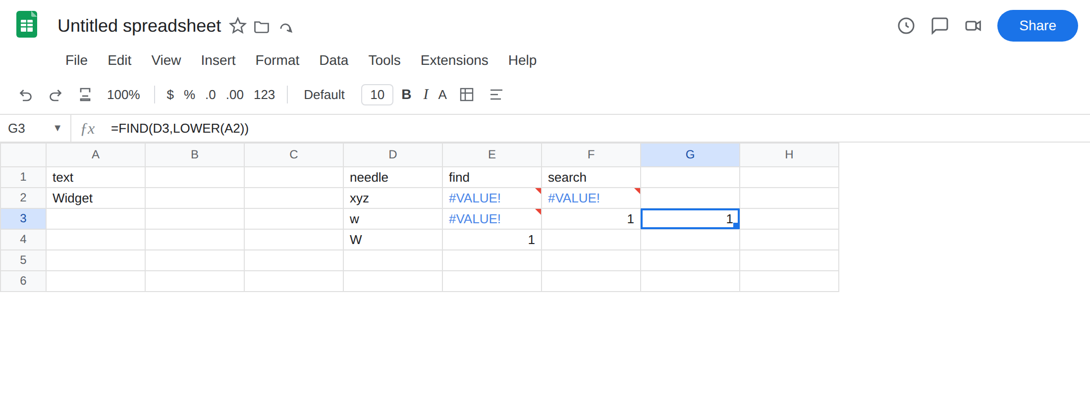
Pick FIND or SEARCH on purpose. Case must match: FIND. Case must not matter: SEARCH. Keep E4 as the FIND("W",A2) hit. For a lowercase needle with FIND, normalize: in G3 enter =FIND(D3,LOWER(A2)). The cell shows 1. Or switch that row to SEARCH.
When a miss is allowed. Wrap with IFERROR only if you understand you are hiding #VALUE! — and any other error. There is no IFNA equivalent here because the error is not #N/A. A tighter guard: =IF(ISNUMBER(SEARCH(D2,A2)),SEARCH(D2,A2),"none"). ISNUMBER is TRUE on a position and FALSE on #VALUE! if you test a working SEARCH in a helper, or use IFERROR(SEARCH(D2,A2),"none") when a miss should print none. See IFERROR vs IFNA — IFNA will not catch this cell.
Do not switch to REGEXEXTRACT to “get #N/A instead.” Different function, different error, different return. If you wanted a regex, go to that page. If you wanted a position, stay on FIND / SEARCH and handle #VALUE!.
If the cell is #VALUE! and the formula is FIND or SEARCH, the substring is not there — or FIND is waiting on a case that SEARCH would ignore.
Why this is #VALUE! not #N/A
Section titled “Why this is #VALUE! not #N/A”#N/A is Sheets’ “no match” for lookups and for functions that return a matched item (VLOOKUP, MATCH, FILTER, REGEXEXTRACT, XLOOKUP). FIND and SEARCH are not lookups. They are position extractors. The successful type is a positive integer. Failure to produce that integer is a value error, the same family as asking VALUE to parse pcs. Excel defined this decades ago as #VALUE!. Sheets keeps that contract so a formula that tests ISNA around FIND never fires, and IFNA never fires either. Test ISNUMBER, or wrap IFERROR, or fix the needle. Do not wait for #N/A on this function pair.