SPARKLINE bar is already stacked; a group option is #N/A

Google’s help defines SPARKLINE chart type bar as a stacked bar. The numbers in the data range become segments of one bar in one cell. There is no option named group, and there is no option named stacked that you add on top. An unknown option is #N/A. The stack never draws. A vertical range such as A2:A4 still fills only the cell that holds the formula. It does not spill a stack down the column. column draws separate columns. It is the type people reach for when they wanted grouped bars side by side, and it is not a stack.

Unknown option names, including a bad color key, are SPARKLINE charttype and SPARKLINE color / rtl. Blanks and #N/A inside the data are SPARKLINE blanks. Keep the Google Sheets UI in English. Sheet Error is an independent formula-error library, not a Google product.

Recreate it on a blank sheet

1. Open a blank spreadsheet. In A1 type a, B1 b, C1 c. A2 2, B2 3, C2 5. In A3 type 2. A4 3. A5 5. Row 2 is the same three numbers written across. Column A from row 3 is those numbers written down.

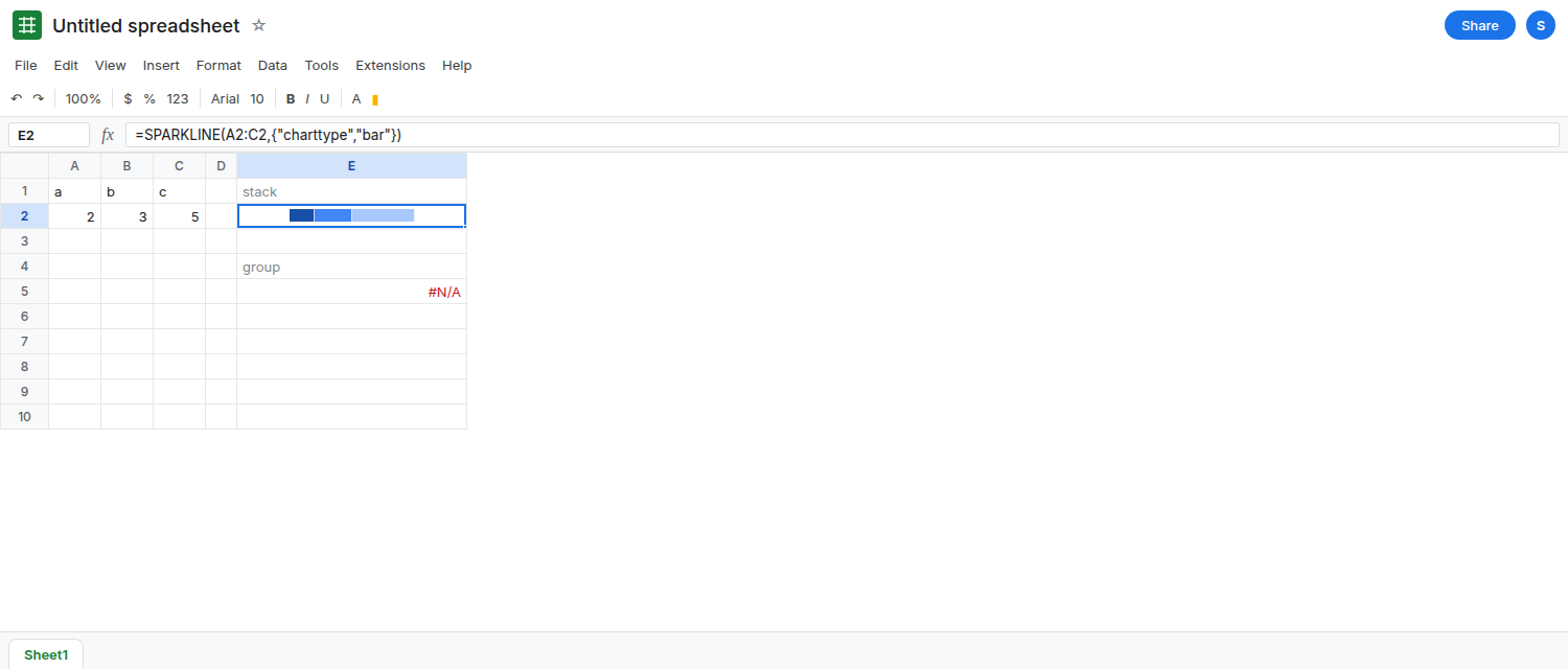
One stacked bar. In E1 type stack. In E2 enter =SPARKLINE(A2:C2,{"charttype","bar"}). E2 shows one horizontal bar made of three segments. No second option. That cell is the control. Bar colors, if you set them, are color1 and color2. See SPARKLINE color / rtl.

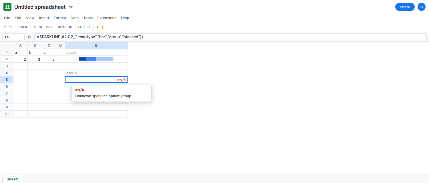
The word group. In E4 type group. In E5 enter =SPARKLINE(A2:C2,{"charttype","bar","group","stacked"}). E5 is #N/A. group is not an option name. Sheets does not ignore the pair and fall back to E2. There is no chart in E5. Leave E5 broken.

A column of numbers does not fill the column with stacks. In E7 type down. In E8 enter =SPARKLINE(A3:A5,{"charttype","bar"}). E8 shows one stacked bar, in E8 only. A3:A5 are the segments. E9 and E10 stay empty. People read that as “the series did not stack down the group.” The function never spills. Leave E8 as that single cell.

column is not a stack. In G1 type cols. In G2 enter =SPARKLINE(A2:C2,{"charttype","column"}). G2 draws separate columns for 2, 3, and 5, not one bar divided into parts. Use it when you wanted side-by-side columns. It will not match E2. Leave G2 as columns.

If { is #ERROR! with Formula parse error, this locale uses \ between array columns. Write {"charttype"\"bar"}. See array literal locale.

What is actually wrong

• bar already means stacked. Adding group or stacked does not switch on a mode. Those names are unknown, and an unknown option is #N/A, the same class as coulour on the color page. E5 is that error. E2 is the stack.
• One formula, one cell. A3:A5 is the data of E8, not a list of sparkline anchors. To get one bar per row you put one SPARKLINE in each row, pointed at that row’s numbers.
• column and bar are different chart types. Grouped columns are column. A single stacked bar is bar. Asking bar for a group of side-by-side bars, or column for one stack, swaps the picture and can look like a broken option.
• Documented bar options include max, color1, color2, empty, nan, and rtl. max sets the scale. It does not group rows. A blank or text cell is empty / nan, and the segment disappears or breaks. See SPARKLINE blanks.

This is not Insert → Chart. A sheet chart can be a stacked column with a series per column. A sparkline cannot.

Fix

Leave E5 as #N/A.

Drop the unknown option. Keep E2: =SPARKLINE(A2:C2,{"charttype","bar"}). One stacked bar of 2, 3, and 5.

One stack per row. Put 2, 3, 5 on row 3 in B3:D3 if you need a second series. In E3 enter =SPARKLINE(B3:D3,{"charttype","bar"}). E3 is that row’s bar. Fill the formula down only when each row has its own three numbers. Filling E2 over a vertical range repeats one range or breaks the references. Check the formula bar after the fill.

Side-by-side columns. Keep G2 when the picture you wanted is columns, not segments. Do not add group to G2. It will #N/A the same way.

Do not wrap E5 in IFERROR. You would hide the bad option and show a blank cell instead of the stack. See IFERROR vs IFNA.

If the cell is #N/A and the option array contains group, delete that pair. If one cell stacks and the rows below stay empty, the data was a vertical range on a single formula. Put a SPARKLINE on each row, or pass a horizontal range.