GETPIVOTDATA returns #REF! when the field or item is gone

GETPIVOTDATA reads one number out of a pivot table by field name and item name. It does not read the cell you clicked as a permanent address. If the pivot no longer has that value field, or the item is filtered out or renamed, the cell is #REF!. The formula bar still shows the old names in quotes. Rebuilding the grid does not update those quotes for you.

This page is that #REF!. It is not VLOOKUP no match (#N/A on a flat list). It is not after you delete (#REF! written into the formula because a cell was deleted). Keep the Google Sheets UI in English.

Recreate it on a blank sheet

1. Open a blank spreadsheet. In A1 type dock, B1 qty. A2 East, B2 10. A3 East, B3 3. A4 West, B4 4. This is the source, not the pivot.

Build the pivot. Select A1:B3 (leave West out for a moment). Insert → Pivot table. Put the pivot on the same sheet, starting at D1. In the pivot editor, add Rows: dock. Add Values: qty, summarized by SUM. D1 is the pivot anchor. You should see East and a sum of 13.

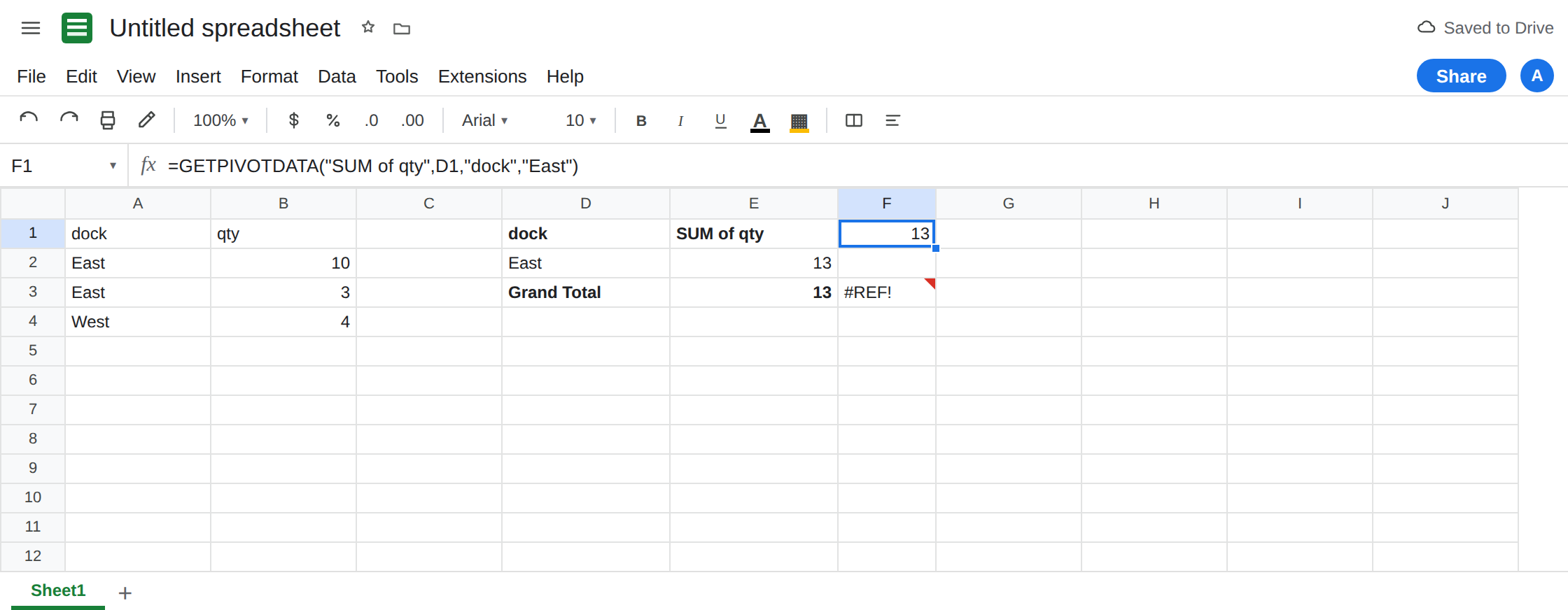
Insert GETPIVOTDATA the way Sheets writes it. Click F1. Type = and then click the East sum cell in the pivot (the 13). Sheets fills GETPIVOTDATA, not =D2 or whatever cell you clicked. The formula looks like =GETPIVOTDATA("SUM of qty",D1,"dock","East"). The value name can be SUM of qty or a close variant depending on the summarizer label. F1 shows 13. That cell is the control. If Sheets inserted a plain =D2 instead, type the GETPIVOTDATA formula yourself with the value name you see in the pivot header.

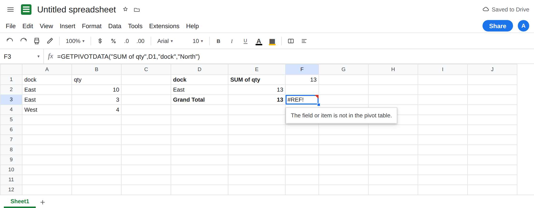
Wrong item. In F3 enter =GETPIVOTDATA("SUM of qty",D1,"dock","North"). North is not a row. F3 is #REF!. The tooltip says the field or item is not in the pivot table. Leave F3 broken.

Item that exists in the source but not in this pivot. In F5 enter =GETPIVOTDATA("SUM of qty",D1,"dock","West"). West is in A4, and A4 was not in the pivot range. F5 is #REF!. The source row is real. The pivot does not know it. Leave F5 broken.

Renamed value field. In the pivot editor, remove the qty value and add it again summarized by COUNTA, or rename the value header if the editor lets you edit the label. The header is no longer the string inside F1’s first argument. F1 flips to #REF! even though a number still sits in the pivot. Put the summarizer back to SUM of qty so F1 returns to 13, and leave F3 as the broken item.

Anchor that is not a pivot. In F7 enter =GETPIVOTDATA("SUM of qty",A1,"dock","East"). A1 is the word dock, not a pivot cell. F7 is #REF!. The second argument must be any cell inside the pivot, usually the corner. Leave F7 broken.

Leave F3, F5, and F7 broken when they are #REF!. Leave F1 as 13 after you restore SUM.

What is actually wrong

• The arguments are labels, not positions. "East" has to match a pivot item. "SUM of qty" has to match the value field’s name as the pivot shows it. A filter that hides East, a row group you removed, or a summarizer you switched from SUM to COUNT changes those labels. The formula does not follow the click you made last week.
• The second argument only locates the pivot. It is not the cell of the answer. Pointing it at the source header is #REF! even when every name is spelled correctly. F7.
• Source rows outside the pivot’s data range do not exist for GETPIVOTDATA. Expanding the pivot to A1:B4 makes West appear. Until you do that, F5 is correct to fail.
• #REF! here is not a deleted A1 on this sheet. The formula text is still a function call with quoted strings. See after you delete.
• A flat SUMIF does not break when you reorder the pivot, because it does not read the pivot. If the question is “qty for East in the source,” SUMIF is the stabler formula. GETPIVOTDATA is for “whatever the pivot currently calls this item.”

This is not QUERY pivot. See QUERY PIVOT. Different function, different column language.

Fix

Leave F3 and F7 broken.

Copy the names from the pivot you have now. Click F1, type =, click the East sum again, and press Enter. Or edit the quoted strings so they match the header and the row label character for character, including SUM of qty versus Sum of qty if that is what the header shows. F1 should be 13.

Widen the pivot data range to A1:B4 if West should be an item, then use "West" in a new formula. Do not point F5 at A4 and expect GETPIVOTDATA to skip the pivot.

If you wanted a normal cell reference, delete the GETPIVOTDATA call and type =D2 (or whichever cell holds the sum). That reference follows the cell. It breaks if you move the pivot. It does not break if you rename a row label in the source and refresh. Pick the one that matches the question.

Do not wrap F3 in IFERROR. A missing item and a broken anchor would both become blank. See IFERROR vs IFNA. IFNA does not catch #REF!.

If GETPIVOTDATA is #REF!, read the quoted field and the quoted item against the pivot on the screen. Then check that the second argument is a cell inside that pivot. The source list can still be right.