Fix #NUM! in Google Sheets

#NUM! means the formula parsed and the argument is a number — just not a number this function can use. The domain is wrong, or the result is larger than Sheets can represent. The type is already numeric.

Recreate it on a blank sheet

Open a blank spreadsheet. In A1 type x, B1 sqrt, C1 ok.
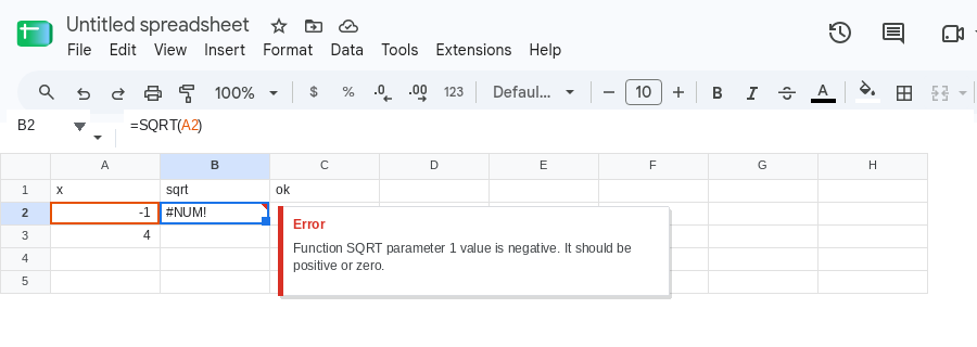
In A2 type -1 as a number. In B2 enter =SQRT(A2). The cell shows #NUM!. The tooltip is Function SQRT parameter 1 value is negative. It should be positive or zero.
In A3 type 4. In C3 enter =SQRT(A3). The cell shows 2. Same function, non-negative input, no error.

Leave B2 as the broken formula.

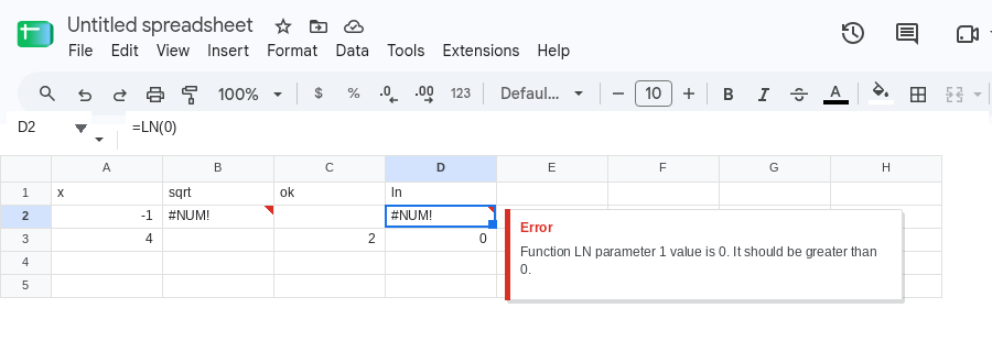
Second recreate — log of zero. In D1 type ln. In D2 enter =LN(0). The cell shows #NUM!. Natural log is not defined at 0. In D3 enter =LN(1). The cell shows 0. That row is the control.

Third recreate — overflow. In E1 type fact. In E2 enter =FACT(171). The cell shows #NUM!. Factorial of 171 is larger than Sheets can store as a number. In E3 enter =FACT(5). The cell shows 120.

SQRT(-1), LN(0), and FACT(171) are three different stories with the same error value: the number is out of domain, or too big.

What is actually wrong

SQRT returns a real square root. -1 is a number. There is no real square root of a negative, so the cell is #NUM!. Sheets does not switch to complex numbers for SQRT.
LN(0) and LOG of 0 or a negative are the same class of failure: the function is defined only for positive numbers.
FACT(171) (and FACT of a negative) is a numeric limit, not a typo. The argument type is still a number.
Other functions follow the same pattern. POWER(10,1000) is #NUM! because the result overflows. An IRR that never settles can also land here. The recreate above is the one you can type in ten seconds.

This is not #VALUE!. #VALUE! is the wrong type — text in a +, VALUE("pcs"), DATEVALUE("Widget"). See wrong type. A2 is the number -1. ISNUMBER(A2) is TRUE. The function refused the domain, not the type.

This is not #DIV/0!. Divide-by-zero is 10/0 or a blank divisor. See divide by zero. SQRT is not division. LN(0) is not 1/0.

This is not #N/A. Nothing is being looked up. See what #N/A means.

This is not #NAME?. SQRT, LN, and FACT are real function names. See unknown function.

This is not a Formula parse error. The formulas parsed. A parse error is #ERROR! from argument separators. See locale parse error.

Excel users sometimes see #NUM! from ROUND with an impossible number of digits. Do not chase that on this sheet. Google Sheets ROUND does not use that Excel failure as its everyday #NUM!. SQRT(-1) is the reliable recreate here.

Fix

Leave B2, D2, and E2 broken so #NUM! stays on the sheet.

Fix the input when the negative is a mistake. If A2 should have been a length, a variance, or a count, put the real non-negative number in A2. B2 becomes a square root and you do not need a wrapper.

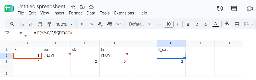
Guard the domain. When a negative (or zero) is possible and should not run the function, test first. In F1 type if_sqrt. In F2 enter =IF(A2<0,"",SQRT(A2)). The cell is empty. In F3 enter =IF(A3<0,"",SQRT(A3)). The cell shows 2. For LN, the test is >0: =IF(A2>0,LN(A2),"").

Absolute value only if you mean magnitude. =SQRT(ABS(A2)) returns 1 for -1. That is correct when you want the root of the size and the sign is noise (a deviation, a difference you already know is a distance). It is the wrong fix when a negative means the model is invalid. Do not hide a bad sign with ABS by default.

Overflow. You cannot factorial-your-way past the numeric limit. If FACT(171) is the formula you typed, you do not need that number in a cell. Scale the model, or compute on the source and import a summary. That is a different “too large” from IMPORTRANGE result too large, which is a transfer cap, not a factorial.

IFERROR. =IFERROR(SQRT(A2),"") clears B2 and also hides #VALUE!, #REF!, and #NAME? if someone later breaks the formula in another way. Use it only when any error should look like “no result.” Prefer the IF on the domain when you care which error you are catching. See IFERROR vs IFNA.

Do not wrap a domain error you have not looked at. If A2 is a formula that should have returned 4 and returned -1, fix that formula. IF will not.