Fix MATCH #N/A in Google Sheets (no match and match type)

MATCH returns the relative position of a key in a range. #N/A means it did not find a position it is allowed to return. That can be a real miss (match_type 0 and the key is absent). It can also be the default approximate match (match_type 1) on a range that is not sorted ascending. Both cells show #N/A. They are not the same problem.

This page is MATCH. It is not an XLOOKUP miss — see XLOOKUP #N/A. It is not VLOOKUP no match (number vs text, a trailing space). It is not what #N/A means as a general primer, though that page is the right start if you only know the error value.

Recreate it on a blank sheet

1. Open a blank spreadsheet. In A1 type sku. In A2 type 101. A3 103. A4 102. The list is not sorted. D1 lookup. D2 999. D3 102.

Exact miss. In E1 type exact. In E2 enter =MATCH(D2,A2:A4,0). The cell shows #N/A. The tooltip is Did not find value ‘999’ in MATCH evaluation. 0 is exact match. 999 is not in A2:A4. Leave E2 broken.

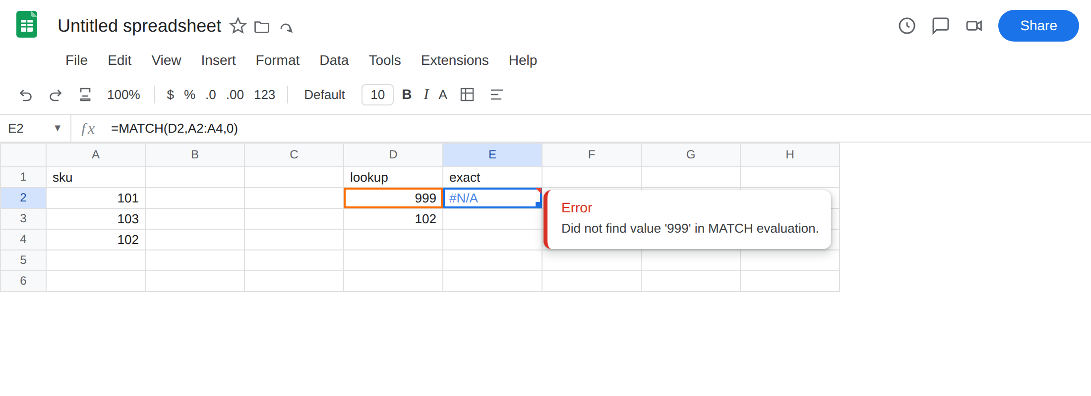
Exact hit on the unsorted list. In E3 enter =MATCH(D3,A2:A4,0). The cell shows 3. Sku 102 is the third cell in A2:A4. Exact match does not care about sort order.

Wrong match_type — default / 1 on unsorted data. In F1 type approx_1. In F2 enter =MATCH(D3,A2:A4,1). 1 is approximate: largest value less than or equal to the key, range must be sorted ascending. A2:A4 is 101, 103, 102. F2 is #N/A or a wrong position — not 3. Omitting the third argument is the same as 1. In F3 enter =MATCH(D3,A2:A4). Compare F3 with F2. Leave both if they are not 3.

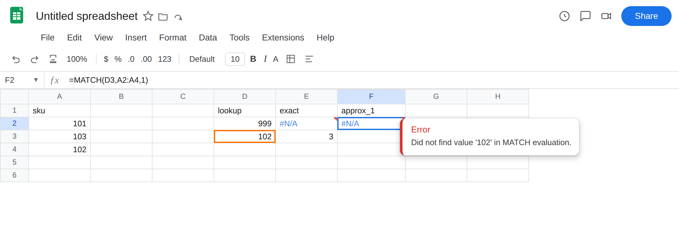
match_type -1 on the same unsorted list. In G1 type approx_-1. In G2 enter =MATCH(D3,A2:A4,-1). -1 is approximate the other way: smallest value greater than or equal, range must be sorted descending. A2:A4 is not descending. G2 is #N/A or a wrong position. Leave G2 broken.

Confirm the exact miss. Type 102 in D2. E2 becomes 3. Put 999 back so #N/A returns. If toggling the lookup value makes #N/A come and go on E2, that cell is a real absence. F2 will not toggle the same way: 102 is on the sheet and approximate match can still fail.

What is actually wrong

• MATCH(key, range, 0) is exact. #N/A means the key is not in the range (or it does not actually match: number vs text, a trailing space). D2 999 is the clean miss.
• MATCH(key, range, 1) — and MATCH with the third argument omitted — is not exact. Sheets assumes A2:A4 is sorted A→Z / small→large. 101, 103, 102 is not. Approximate match then returns #N/A or a surprising index. That is not “102 is missing.”
• MATCH(key, range, -1) assumes descending sort. The same unsorted column fails that contract too.
• The result is a position, not a name. 3 means the third cell of A2:A4. People wrap INDEX around it (=INDEX(B2:B4,MATCH(D3,A2:A4,0))) to pull a column. The #N/A still comes from MATCH. Fix MATCH first.
• Number vs text still misses with 0. Text '102 versus numeric 102 is VLOOKUP no match on a different function. LEN / ISNUMBER is the check. Changing match_type will not coerce types.

This is not XLOOKUP / VLOOKUP returning a value from another column. Those pages: XLOOKUP #N/A, VLOOKUP no match, XLOOKUP vs VLOOKUP. MATCH only tells you where the key sits.

This is not FILTER with zero rows. See FILTER no match.

Fix

Leave E2 as the exact miss. Leave F2 and G2 as the approximate failures.

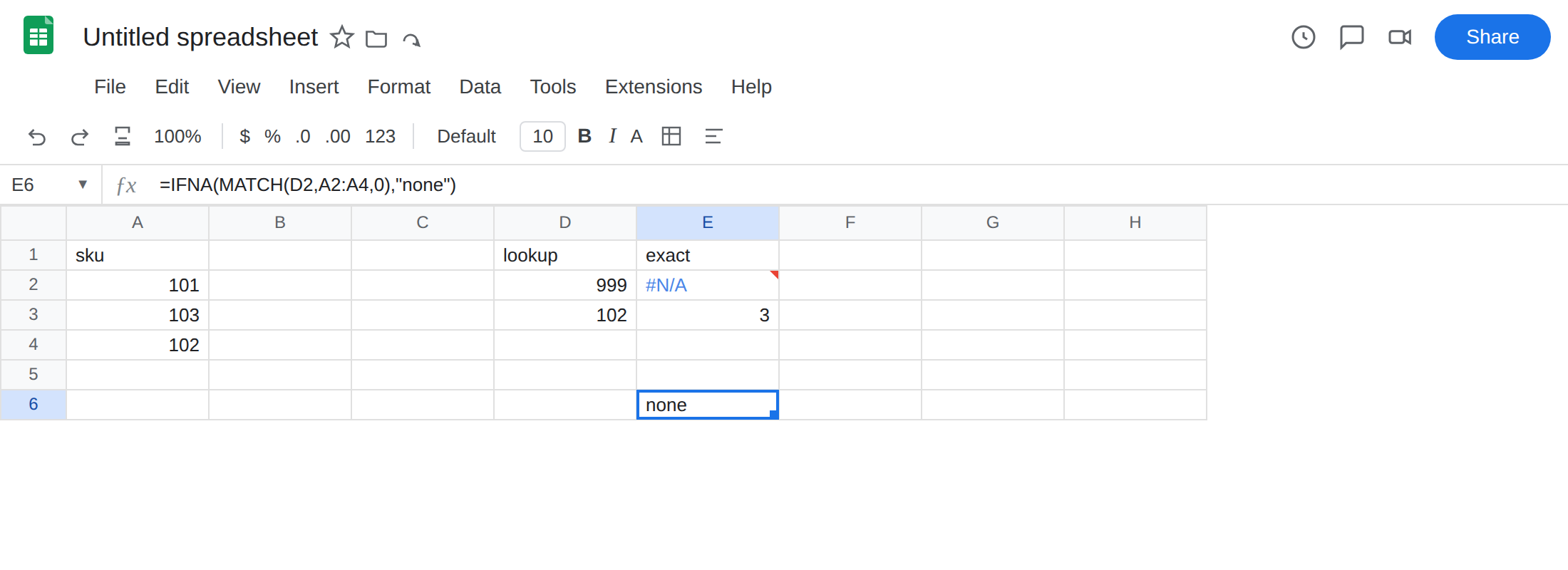
Sku lookups: pass 0. Keep E3: =MATCH(D3,A2:A4,0) returns 3. For a miss that is allowed to print a label, wrap only the exact form: in E6 enter =IFNA(MATCH(D2,A2:A4,0),"none"). The cell shows none. Use IFNA, not IFERROR. See IFERROR vs IFNA. Do not wrap F2. Approximate #N/A on an unsorted list is a match_type bug, not a missing sku.

If you actually want a band. Sort the range the way that match_type requires, then use 1 or -1 on purpose (tax bracket, quantity break). Do not sort a sku list to make the default look right. Sku lists use 0.

Do not omit the third argument on a sku. =MATCH(D3,A2:A4) is 1. Type the 0.

If MATCH is #N/A and you can see the key, read the third argument before you rewrite the table. 0 plus a visible key is type or spaces. 1 or omitted on an unsorted column is this page.

MATCH vs XMATCH

XMATCH is the newer sibling. Default match_mode is exact, the same idea as XLOOKUP defaulting to exact. MATCH’s default is still approximate 1. If you are writing a new position formula and you want exact sku behavior without remembering to type 0, XMATCH(D3,A2:A4) returns 3 on this unsorted list. This page stays on MATCH: pass 0, or sort only when you mean approximate. Do not migrate a working MATCH(...,0) just to clear #N/A from a 999 that is not in the column — that miss is correct.