Fix TO_PURE_NUMBER on currency and text in Google Sheets

TO_PURE_NUMBER(value) takes a numeric cell (currency, percent, date, duration) and returns the same number with ordinary number formatting. It does not parse a string that looks like money. Text is returned unchanged. Arithmetic on that leftover text is then #VALUE!. VALUE() is the parser for numeric text. N() turns non-numbers into 0 (except TRUE → 1).

This page is TO_PURE_NUMBER on format vs text. It is not VALUE() locale (VALUE("1.234,56") on a US sheet). It is not wrong type as a generic 10 + pcs primer, though that is the arithmetic you hit after a passthrough. Keep the Google Sheets UI in English.

Recreate it on a blank sheet

1. Open a blank spreadsheet. File → Settings → Locale → United States. In A1 type kind, B1 raw, C1 pure, D1 plus1.

Formatted currency (numeric). In A2 type fmt. In B2 type 12.5. Format B2 as Format → Number → Currency. B2 displays $12.50 (or similar) and ISNUMBER(B2) is TRUE. In C2 enter =TO_PURE_NUMBER(B2). C2 is 12.5 with no currency format. In D2 enter =C2+1. The cell shows 13.5. That row is the control: format stripped, math works.

Currency as text. In A3 type text. In B3 type an apostrophe then $12.50 so the cell is text. ISTEXT(B3) TRUE. In C3 enter =TO_PURE_NUMBER(B3). C3 is still $12.50. No #VALUE! from TO_PURE_NUMBER itself. In D3 enter =C3+1. D3 is #VALUE!. Tooltip: expects number values. The convert “failed” by doing nothing.

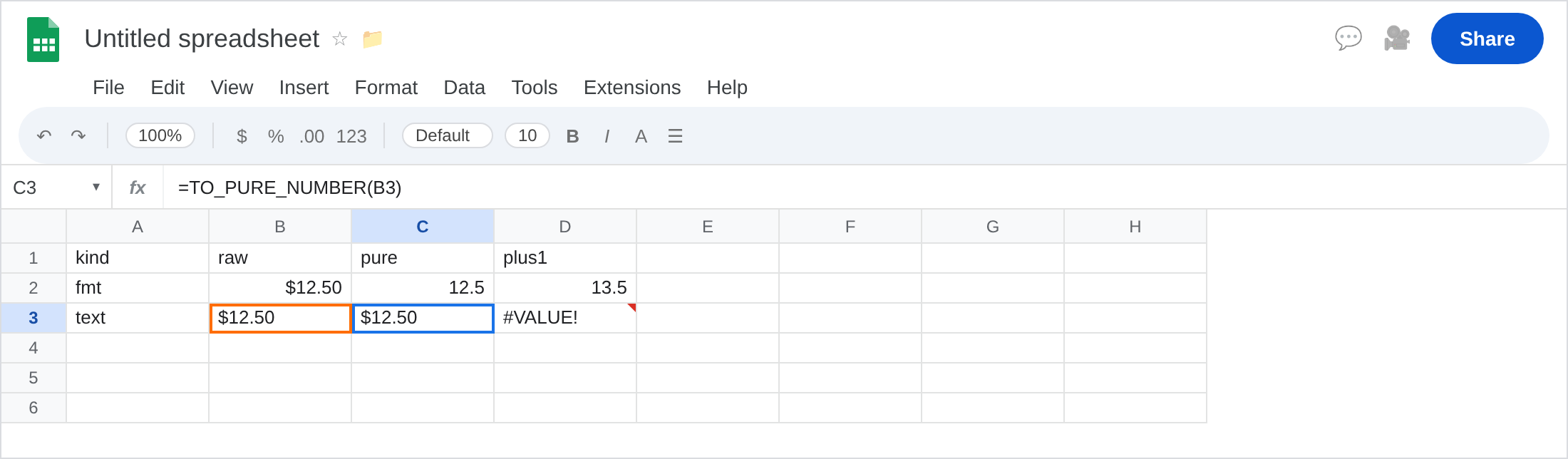
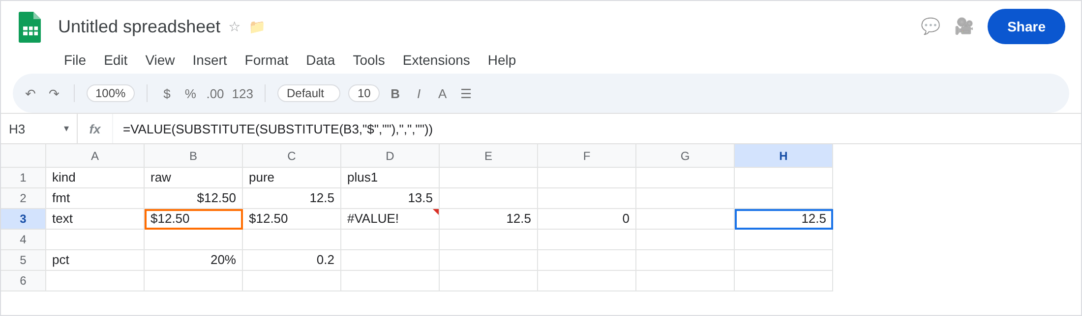
VALUE on the same text (contrast). In E3 enter =VALUE(SUBSTITUTE(B3,"$","")). On United States this often becomes 12.5. VALUE(B3) may already coerce $12.50 on a US locale; if E3’s extra SUBSTITUTE is needed, keep it. Leave D3 broken. The locale-shaped parser page is VALUE() locale.

Percent format. In A5 type pct. In B5 type 0.2. Format as Percent (20%). In C5 enter =TO_PURE_NUMBER(B5). C5 is 0.2, not 20. That is success. People who expected 20 wanted B5*100, not TO_PURE_NUMBER.

N() contrast. In F3 enter =N(B3). Text becomes 0. Silent zero, not passthrough. Different hazard. Leave F3 as 0 so you can see why N is not a fix for $12.50 text.

Leave C3 as passthrough text. Leave D3 as #VALUE!. Leave C2 as the working pure number.

What is actually wrong

• TO_PURE_NUMBER is Format → Number → Number as a function. It needs ISNUMBER. Display $ on a numeric cell is format, not the character $.
• Apostrophe $12.50 is four-to-six characters of text. The function copies them. The red triangle shows up on the next math, not on C3.
• N(text) is 0, which will not #VALUE! on +1 — you get 1 and a wrong total. Do not swap N in to “fix” C3.
• Percents are stored as fractions. Pure number of 20% is 0.2. Currency of 12.5 is 12.5. Dates become serials (see TO_DATE for the inverse).

This is not DATEVALUE of 13/1/2024. See DATEVALUE locale.

This is not SUMIFS skipping date text. See SUMIFS date text.

This is not CSV sku number-vs-text in a lookup. See CSV text vs number.

Fix

Leave D3 broken so the delayed #VALUE! stays visible.

If the cell is already numeric, keep C2. Change format on B2, or use TO_PURE_NUMBER when you must pass a raw number into a system that hates $.

If the cell is text, parse it. In H3 enter =VALUE(SUBSTITUTE(SUBSTITUTE(B3,"$",""),",","")). Then H3+1 is 13.5. Confirm with ISTEXT(B3) before you choose TO_PURE_NUMBER vs VALUE.

Do not wrap D3 in IFERROR until you know C3 is text. See IFERROR vs IFNA. IFNA will not catch #VALUE!.

If TO_PURE_NUMBER equals the source and ISTEXT is TRUE, you needed VALUE (or SUBSTITUTE then VALUE). If ISNUMBER is TRUE and you still see $, that is format on the source cell — C2 already stripped it.

Format vs text vs N()

Formatted $12.50 (number) → TO_PURE_NUMBER → 12.5. This page’s success row.

Typed $12.50 (text) → passthrough → +1 is #VALUE!. Parse with VALUE.

N("anything") → 0. Looks numeric, kills the amount. Use N only when you truly want “non-number = 0.” VALUE() locale failures (European 1.234,56 on a US file) are the next tutorial, not TO_PURE_NUMBER.