Clicking a pivot cell inserts GETPIVOTDATA, which breaks when the labels change

Start a formula with = and click a value inside a pivot table. Google Sheets does not insert =E3. It inserts GETPIVOTDATA with the value field’s name, the pivot’s anchor, and the row or column item you clicked. The formula follows those labels. It does not follow the cell. Change the summarizer, remove the row field, or filter that item out, and the formula is #REF! even though a number still sits in the pivot. A cell reference you type yourself keeps showing whatever number later lands in that cell, which may be a different item.

A #REF! because the item or the field string is already wrong is GETPIVOTDATA. Grouped dates, whose item labels are not the original day, are GETPIVOTDATA month. Keep the Google Sheets UI in English. Sheet Error is an independent formula-error library, not a Google product.

Recreate it on a blank sheet

1. Open a blank spreadsheet. In A1 type dock, B1 qty. A2 East, B2 10. A3 East, B3 3. A4 West, B4 4. East’s sum is 13. West’s is 4.

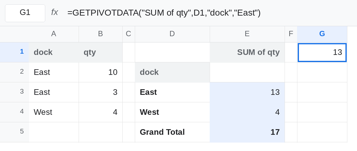
Build the pivot. Select A1:B4. Insert → Pivot table. Put it on the same sheet, starting at D1. Rows: dock. Values: qty, summarized by SUM. You should see East 13 and West 4. Note the cell that shows 13. On a pivot starting at D1 it is often E3, under a header like SUM of qty. Call that cell the East total for the rest of this page. The anchor of the pivot is D1.

Click, do not type the address. Select G1. Type = and then click the East total. Press Enter. The formula bar shows GETPIVOTDATA, with a first argument like "SUM of qty", a second argument of D1, then "dock" and "East". G1 is 13. It is not =E3. If your click inserted a plain cell reference, you clicked a header or a cell outside the value grid. Click the 13 again. That generated formula is the control: right number, labels stored as text.

A typed address follows the cell, not East. In G3 type = and then type the address of the East total yourself, for example =E3, without clicking. G3 is 13. In the pivot editor, drag the row order so West is first, or sort the dock field descending if the editor offers sort. The 13 moves to a different row. G1 still shows 13, because it still asks for East. G3 shows whatever number now sits in E3, which can be West’s 4. Neither cell errored. They stopped agreeing. Put the sort back so East is the first data row again before the next step.

Change the label the formula quoted. In the pivot editor, remove qty from Values and add it again summarized by COUNTA, or edit the value header so it no longer reads the string inside G1. G1 flips to #REF!. The tooltip says the field name is not in the pivot. G3, the typed address, still shows a number: the count of qty rows now sitting in that cell. The grid is fine. The generated formula is quoting a header that no longer exists. Restore SUM of qty so G1 returns to 13.

Remove the row field the formula quoted. Remove dock from Rows. The pivot may collapse to a single grand total. G1 is #REF! again, because "dock" / "East" is not an item layout anymore. G3 still shows the number in that cell. Add dock back as a row so G1 works. Then use the pivot’s filter to hide East only. G1 is #REF! while West remains. The click you made last week did not store “the cell I was looking at.” It stored the item name East.

Leave G1 as #REF! while East is filtered out, or restore East and leave G1 as 13 with G3 still a raw address so both styles stay on the sheet.

What is actually wrong

• The click writes a label query. "SUM of qty" must match the value header. "East" must match a pivot item. "dock" must still be a row or column field. The second argument only finds the pivot. It is the anchor, not the answer cell.
• Sorting or rearranging items does not break GETPIVOTDATA. It breaks a raw address. G1 staying on 13 while G3 flips to 4 is the feature, and it is why Sheets inserts the function.
• Renaming the summarizer, removing the field, or filtering the item out breaks GETPIVOTDATA and does not blank the pivot. The #REF! is the formula. See GETPIVOTDATA for a wrong item that was never in the pivot, which is the same token for a different edit.
• Google Sheets has no checkbox that turns this click behavior off. Excel does: on the PivotTable Analyze tab, open the Options menu and clear Generate GetPivotData. After that, a click in Excel inserts a cell reference. That toggle is not in the Sheets pivot editor. Typing the address is how you opt out in Sheets.
• Copying G1 and changing "East" to "West" is still a label query. It works while West is visible and #REF!s when West is filtered. It does not become “whatever is in the cell below.”

This is not a deleted cell on the sheet. The formula text is still GETPIVOTDATA. See after you delete.

Fix

Leave one broken generated formula on the sheet if East is filtered out, so the #REF! stays visible. Restore the East row when you want G1 to calculate.

Keep GETPIVOTDATA when the question is the item. G1 is the right formula for “East’s sum, even if the pivot is sorted.” When you change the summarizer, edit the first quoted string to the new header, or click the value again into an empty cell and compare. Date groups need the group label, not the original day. See GETPIVOTDATA month.

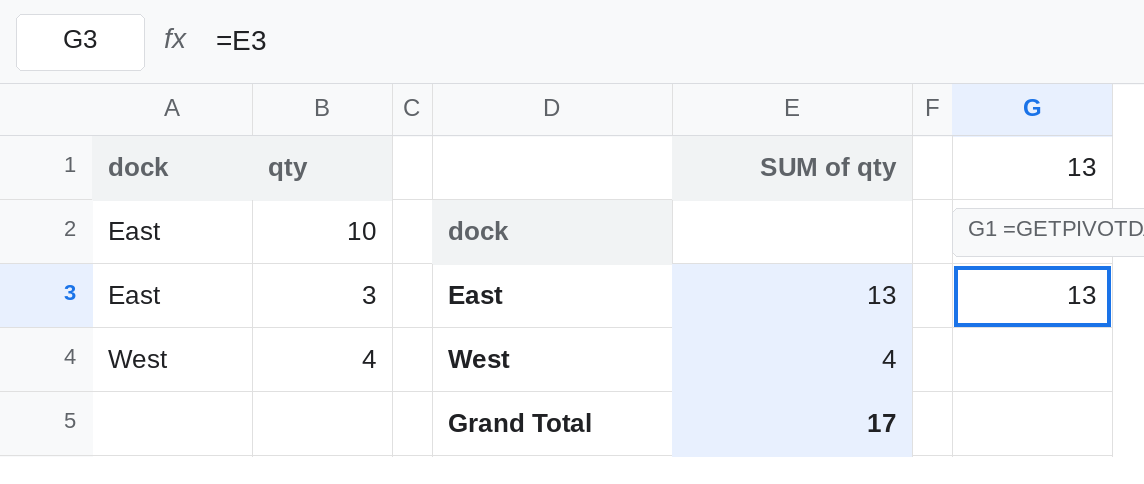
Type the address when the question is the grid cell. Use G3’s style, =E3, for “whatever this pivot cell shows after the next layout change.” Do not start with = and click, or Sheets will replace your intention with labels. If the next change moves East to another row, update the address, or go back to GETPIVOTDATA on purpose.

A source total does not use the pivot. =SUMIF(A2:A4,"East",B2:B4) is 13 and does not care about the pivot editor. Use it when the pivot is only a view and the contract is the source column.

If the formula appeared the moment you clicked, you did not choose GETPIVOTDATA from memory. The labels inside the quotes are the contract. If those labels still match the editor, a #REF! is a filtered or removed item, not a bad click. If you needed the cell to follow the grid, replace the function with an address you type.